Characteristics Collocation Method of Compressible Miscible Displacement with Dispersion

(1)

http://dx.doi.org/10.4236/jamp.2015.31012

Characteristics Collocation Method of

Compressible Miscible Displacement with

Dispersion

Ning Ma, Xiaofei Lu

College of Science, China University of Petroleum, Beijing, China Email: [email protected]

Received December 2014

Abstract

The compressible miscible displacement in a porous media is considered in this paper. The prob-lem is a nonlinear system with dispersion in non-periodic space. The concentration is treated by a characteristics collocation method, and the pressure is treated by an orthogonal collocation me-thod. Optimal order estimates are derived.

Keywords

Compressible, Dispersion, Characteristics Collocation, Non-Periodic

1. Introduction

The mathematical controlling model for compressible miscible displacement in porous media with dispersion is given by

( ) p ( ) p [ ( ) ] , ( , ) , (0, ]

d c u d c a c p q x y t T

t t

∂ _{+ ∇ ⋅ =} ∂ _{− ∇ ⋅} _{∇ =} _{∈ Ω ∈}

∂ ∂ (1)

( ) ( ( ) ) ( ) , ( , ) , (0, ].

c p

b c u c D u c c c q x y t T

t t

ϕ∂ + ∂ + ⋅∇ − ∇ ⋅ ∇ = − ∈ Ω ∈

∂ ∂ (2)

where c=c₁= −1 c₂, a c( )=a x y c( , , )=k x y( , ) / ( ),µ c

2 1 1

1

( ) ( , , ) ( , ) { _j _j},

j

b c b x y c

ϕ

x y c z z c

=

= = −

∑

2

1

( ) ( , , ) ( , ) j j.

j

d c d x y c

ϕ

x y z c

=

= =

∑

c_j and z_j denote the concentration and constant compressibility factor for

the i component of the fluid mixture respectively. Let Ω =(0,1) (0,1)× with the boundary ∂Ω, p x y t( , , ) the pressure in the mixture, u is the Darcy velocity of the fluid, and c x y t( , , ) is the relative concentration of the injected fluid. k x y( , ) and ϕ( , )x y are the permeability and the porosity of porous media, µ( )c is the vis-cosity of the fluid. D u( ) ϕ{dm I |u| (d E ul ( ) d Et ( ))}u

⊥

(2)

terms, where dm,d dl, t are the molecular dissipation, longitudinal and tangential dispersion coefficients. I is a 2

unit matrix, 2

2 2

( ) ( k l/ | | )

E u = u u u × is a matrix representing orthogonal projection along the velocity vector and

( ) ( )

E⊥ u = −I E u is the complementary projection. q and c etc. refer to the definition and significance of [1] [2].

We shall assume that no flow occurs across the boundary

0, ( ) 0 , ( , ) ,

u v = D u ∇ ⋅ =c v x y ∈ ∂Ω (3) where v is the outer normal to ∂Ω, and the initial conditions are

0 0

( , , 0) ( , ), ( , , 0) ( , ), ( , ) ,

p x y = p x y c x y =c x y x y ∈ Ω (4)

The compressible flow problems are strongly nonlinear coupling system for partial differential equations of two different types, and we consider the system with dispersion in non-periodic space, so these factors lead to many difficulties for convergence analysis of algorithms. The collocation methods are widely used for solving practice problems in engineering due to its easiness of implementation and high-order accuracy. But the most parts of mathematical theory focused on one-dimensional or two-dimensional constant coefficient problems [3] [4]. [5] proposes the collocation method of two-dimensional variable coefficients elliptic problems. The charac-teristics collocation scheme for the incompressible flow is given in [6]. The characcharac-teristics finite element me-thod for the compressible miscible flow is proved in [7]. In the paper we shall use different technique to treat different types of equations, the orthogonal collocation methods solve the pressure equation and the characteris-tics collocation scheme approximate the concentration equation. We develop some technique to analyze con-vergence of these algorithms for this strongly nonlinear system with dispersion in non-periodic space. Finally we can obtain the optimal order error estimate. We shall assume the coefficients a c D u b c( ), ( ), ( ), ϕ( , ), ( )x y d c

etc. and their partial derivatives have positive upper and lower bounds independently as well as smoothly. Throughout, the symbols K and

ε

will denote, respectively, a generic constant and a generic small positive constant.

The organization of the rest of the paper is as follows. In Section 2, we will present the formulation of the characteristic collocation scheme for nonlinear system (1) (2). In Section 3, we will analyze convergent rate of the scheme defined in Section 2.

2. Characteristic Collocation Scheme (CCS)

2.1. Preliminaries

In this subsection, we will give some basic notations and definition for the characteristics collocation methods, which will be used in this article. We make the partition of the domain Ω, which is quasi-uniform and equally spaced rectangular grid by h_x and h_y steps along x-direction and y-direction. Let

0 1

: 0 1;

x

x x x xN

δ = < << =

δ

y

: 0

=

y

0

< < <

y

1



y

Ny

=

1,

h

x

= −

x

i

x

i−1

,

h

y

=

y

j

−

y

j−1

,

{

}

1 1

max _x, _y , _ij ( _i _i) ( _j _j),

h= h h Ω = x₋ −x × y₋ −y

[0,1],

i

[

₁

],

j

[

₁

]

x i i y j j

I

=

I

=

x

₋

−

x

I

=

y

₋

−

y

.

Define function spaces as follows:

(

)

{

( )

}

(

)

{

(

)

}

1

1 3

1, 1

3, | , 1

3, 3, , (0) (1) 0)

i

x x x

P x x

m v C I v P I i N

m v m v v

δ

δ δ

= ∈ ∈ =

= ∈ = =

 ,

where P₃ denotes the set of polynomials of degree ≤3, similarly we can define m1

( )

3,

δ

y ,m1,P

( )

3,

δ

y . Let

( )

(

)

( )

(

)

( )

1 3, 1 3, x 1 3, y , 1,P 3, 1,P 3, x 1,P 3, y ,

m

δ

=m

δ

⊗m

δ

m

δ

=m

δ

⊗m

δ

then let m₁

(

3,δ

)

be the spaces of piecewise Hermite bicubics.

Next, we take four Gauss points as collocation points in Ωij:

(

ξ ξ

ikx, jly

)

, ,k l=1, 2, and 1

x

ik xi hx k

ξ = − + ξ ,

1 y

jl

y

j

h

y l

(3)

( )

(

)

( )

2

1 1 1 1 , 1

2

1 1 1

2

1 1 1

1 , , , , 4 , , , 2 , , , 2 y y x x x x y y N N N N x y x y ik jl ij

i j i j k l

N N

x x

ik

x ix

i i k

N N

y y

jl

y jy

j j l

u v u v h h uv

h

u v u v uv

h

u v u v uv

ξ ξ

ξ

= = = = = = = = = = = = = = = = =

∑∑

∑

∑ ∑

∑

∑ ∑

( )

1 0 2 1 1 2 1 0 0 1 1 2 1 0 0

, , ,1 , ,1 , , ||| |||

||| ||| , , , 3, ||| ||| , , , 3,

x y y x

x x _y y y

H x

E x x y y y x

u v u v u v u u u

u Du u dx Du u dy u m

u u u dx u u dy u m

δ δ Ω = = = = + ∀ ∈ = + ∀ ∈

∫

Let T_3,δ ∈m₁

( )

3,

δ

be the interpolation operator of piecewise Hermite bicubics on Ω, and T3,δx∈m1

(

3,

δ

x

)

and _3, ₁

(

3,

)

y y

T δ ∈m δ be the interpolation operators of piecewise Hermite bicubics in x and in y, respectively, which may be defined by

T v

_3,_δ

=

T

_3,_δ_x

T

_3,_δ_y

v

=

T

_3,_δ_y

T

_3,_δ_x

v

for sufficiently smooth function v.

2.2. CCS

In this subsection we will present the fully discrete characteristic collocation scheme for nonlinear system (1) (2) with dispersion term in non-periodic space. At first time

[0, ]

T

can be discretized: 0 1

0=t < <t <tn =T,

1

.

n n

t t t −

∆ = − We consider the concentration Equation (2), let

1

2 2 2 ₂

1 2

u

ψ

=



_

ϕ

+ +



_

, and the characteristic

di-rection associated with the operator ϕ + ∇c_t u c is denoted by τ( , )x y , hence c c u c t

ψ ϕ

τ

∂ ₌ ∂ _{+ ∇}

∂ ∂  .

The Equation (2) can be put in the form

( ) ( ( ) ) ( ) , ( , ) , (0, ].

c p

b c D u c c c q x y t T

t ψ

τ

∂ ₊ ∂ _{− ∇ ⋅} _{∇ =} ₋ _{∈ Ω ∈}

∂ ∂ (5)

For (5), we use a backward difference quotient for c τ ∂

∂ along the characteristic line:

1 2

1 1

2 2

( , ) ( , ) 1 | | /

n n n n n

c c x y c x y c c

t

t u

ψ ψ ϕ

τ _ϕ − − ∂ _≈ − ₌ − ∂ _∆ _₊ _ ∆      (6)

where ( , , ), 1 1 , 1 2

n n

n n n n n n u n u

f ft x y t x x t y y t

ϕ

− −

= = − ∆ = − ∆

 _{ } _ _

.

So we can obtain the following discrete equation:

1 1

1 1 1

( ) ( ( ) ) ( ) 0, 1, 2 .

n n n n

n n n n n

h h

h h h h

c c P P

b c D u c c c q n

t t

ϕ

− − ₊ − − − _{− ∇ ⋅} _∇ ₋ − ₋ − ₌ ₌

∆ ∆





Now that use the interpolation operator T_3,_δ and the Gauss points

(

x, y

)

ik jl

ξ ξ

, we give the fully discrete cha-racteristics collocation scheme (CCS):

0 0

3, 0

( , ),

3, 0

( , ),

C

=

T c x y P

_δ

=

T p x y

_δ (7)

1

1 1

( ) ( ( ) ) ( , ) 0,

n n

n n n x y

ik jl

P P

d C a C P q

t

ξ ξ

−

− −

 − _{− ∇ ⋅} _∇ ₋  ₌

 _∆ 

  (8)

1 1

1 1 1

( ) ( ( ) ) ( ) ( , ) 0,

n n n n

n n n n n x y

ik jl

C C P P

b C D U C C C q

t t

ϕ

− − − − −

ξ ξ

 − ₊ − _{− ∇ ⋅} _∇ ₋ ₋  ₌

 _∆ _∆ 

(4)

and 1

( )

n n n

U = −a C − ∇P (10) for 1≤ ≤i Nx,1≤ ≤j Ny, ,k l=1, 2, computed in the order: at first

n

[image:4.595.116.529.263.330.2] [image:4.595.218.413.559.710.2]

P

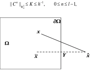
can be computed from (8), then from (10) and (9) we can solve Cn. Because the system is non-periodic, we need to do a continuation as shown in

Figure 1.

We can understand the following method intuitively from above schematic diagram. When xˆ is through the boundary ∂Ω, we will do continuation according to specular reflection method, namely when xˆ is outside Ω, we do the normal from xˆ to ∂Ω, and the normal intersects ∂Ω at Y . Then we do inner normal at Y , and we choose point x so as to xY = xYˆ , and the value of c x( ) replaces the one of c x( )ˆ , in this way c and C etc. functions are certain meaning. Because c satisfies (3), the continuation is logical [7].

3. Convergence Analysis

In this section we consider the existence and uniqueness of the numerical solution, and obtain the optimal error estimate. CCS (8) (9) can be rewritten as the discrete Galerkin method given by [3] [6] [8]

( )

1

1 1

1,

( ) ( ( ) ) , 0, 3,

n n

n n n

P

P P

d C a C P q m

t

χ

δ

−

− − _{− ∇ ⋅} − _∇ ₋ ₌ _{∀ ∈}

∆ (11)

( )

1 1

1 1 1

1,

( ) ( ( ) ) ( ) , 0, 3,

n n n n

n n n n n

P

C C P P

b C D U C C C q Z Z m

t t

ϕ

− − ₊ − − − _{− ∇ ⋅} _∇ ₋ − ₋ − ₌ _{∀ ∈}

δ

∆ ∆ (12)

We can get the following convergence conclusion for the above numerical Scheme (11) (12). Theorem 3.1 Suppose ∆ =t o h( ), then there exists a constant K such that, for h sufficiently small,

/

2 2 2 8

0 ₀

max || || || || ( ).

T t

n n n n

n _n

c C p P t K t h

∆

 

≤ ≤_{ } − +

∑

₌ − ∆ ≤ ∆ +

Proof: Let c=T c_3,_δ ,ξ= −c C,ζ = −c c p , =T_3,_δp,π = −p P,η= −p p. Subtracting (11) from the discrete Galerkin scheme of (1), we obtain the pressure error equation

( )

1 1

1

1,

( ) , ( ( ) ), [ ( ) ( )] , ( ) ,

( )( ), ( ( ) ), [( ( ) ( )) ], , 3,

n n n n

t

n n n n n

t t

n

n n n n

t

n n n

P

d C d a C

d C d c d p d c d

p

d c d p a c

t

a c a C p m

π χ π χ

χ η χ

χ χ δ

− −

−

〈 〉 − 〈∇ ⋅ ∇ 〉

= 〈 − 〉 − 〈 〉

∂

+〈 − 〉 + 〈∇ ⋅ ∇ 〉

∂

+〈∇ ⋅ − ∇ 〉 ∀ ∈



(13)

where

1 n n n

t

f f

d f

t

− − =

∆ , and choosing the test function χ π= n in (13), and the right terms can be denoted by '_, _{1, 2,} _{, 5}

i

T i=  in turn. For error estimate, we shall need an induction hypothesis. We assume that

1

||

n

||

,

0 1,

W

C

K

h

n l

∞

−

≤ ≤

≤ ≤ −

(14)

(5)

We start this induction by seeing that 1 1 1 1

0 0 0 0 1

||

W W W W

C

c

ξ

c

K

h

∞ ∞ ∞ ∞

−

≤



+

≤



≤ ≤

for h sufficiently small.

We shall check that if n=l, (14) is right at the end of the proof. So we get the error estimate of the pressure [6] [8].

1 1

' 2 2 2 8 2 2

* * 1

1 1 1

|| || || || || || ( || || ),

m m m

n m n n

n n n

d

π

t d

π

t K h t

ξ

t

− −

= = =

∆ + + ∇ ∆ ≤ + ∆ + ∆

∑

(15)

for ε sufficiently small.

Next we will consider the concentration equation, subtracting (12) from the discrete Galerkin scheme of (2), 1

1 1 1 1 1

1

1 1 1 1

, ( ( ) ),

ˆ ˆ

, , ,

, ( ( ) ), [ ( ) ( )] ,

[ ( ) ( )] , ( ) ( )

n n

n n n n n n n

n n

n n n n n

n n n

n n n n n n

Z D U Z

t

c c c c c

u c Z Z Z

t t t t

Z D U Z D u D U c Z

t

P P p

c c q Z b C b c

t

ξ

ϕ

ξ

ϕ

ζ

ϕ

ζ

ξ

ζ

−

− − − − −

−

− − − −

− _{− ∇ ⋅} _∇

∆

∂ − − −

= − + ⋅∇ − + −

∂ ∆ ∆ ∆

−

− + 〈∇ ⋅ ∇ 〉 + 〈∇ ⋅ − ∇ 〉

∆

− ∂

+〈 − + + − 〉 + 〈 −

∆ ∂

 

( )

1,

,Z Z mP 3,

t 〉 ∀ ∈

δ

(16)

To obtain optical estimate for

ξ

we choose n

Z=ξ as test function in (16), and we denote the resulting right-hand side terms by T_i ,i=1, 2,,8. And we need another induction hypothesis, we assume that

|| n|| , 0 1

L

P ∞ K n l

∇ ≤ ≤ ≤ − (17)

If l=1, we can start the induction by (15) to get

||

P

0

||

_L

||

p

0

||

_L

||

π

0

||

_L

K

Kh

1

(

h

4

t)

K

∞ ∞ ∞

−

≤ ∇



+ ∇

≤ +

+ ∆ ≤

,

for h sufficiently small and ∆ =t o h( ). We shall check that if n=l, (17) is right at the end of the proof. Simi-lar to the discussion in [6] [8], and the relations (15) (17) and Gronwall lemma, we can get

2 2 8

1

max ||

||

(

).

n

n m

ξ

K

t

h

≤ ≤

≤

∆ +

And it can be combined with (15) to show that

/

2 2 8

1

|| || ( )

T t n

n

t K t h

π

∆

=

∆ ≤ ∆ +

∑

.

At last we shall check the induction hypotheses (14) and (17)

1 1 1

2 1 1 4 1

1 1 4

|| || || || || || || || ( ( )) ,

|| || || || || || || || ( ) ,

l l l l

W W W

l l l l

L L L

C c K Kh h Kh Kh t h h

P p K Kh K Kh t h K

ξ ξ

π π

∞ ∞ ∞

− − − −

− −

≤ + ≤ + ≤ + ∆ + ≤

∇ ≤ ∇ + ∇ ≤ + ∇ ≤ + ∆ + ≤

 

for h sufficiently small , and the proof is complete.

Acknowledgements

We thank the fund “Basic Subjects Fund of China University of Petroleum (Beijing) (KYJJ2012-06-04)”.

References

[1] Douglas Jr., J. and Roberts, J.E. (1983) Numerical Methods for a Model for Compressible Miscible Displacement in Porous Media. Math. Comp., 41, 441-459. http://dx.doi.org/10.1090/S0025-5718-1983-0717695-3

[2] Russell, T.F. (1985) Time Stepping along Characteristics with Incomplete Iteration for a Galerkin Approximation of Miscible Displacement in Porous Media. SIAM. J Numer. Anal., 17, 970-1013. http://dx.doi.org/10.1137/0722059

[3] Dougals, J. and Dupont, T. (1974) Lecture Notes in Math. Vol. 385, Springer-Verlag, Berlin.

(6)

http://dx.doi.org/10.1002/num.1690090207

[5] Bialecki, B. and Cai, X. (1994) H1-Norm Error Bounds for Piecewise Hermite Bicubic Orthogonal Space Collocation Schemes for Elliptic Boundary Value Problems. SIAM. J Numer.Anal., 31, 1128-1146.

http://dx.doi.org/10.1137/0731059

[6] Ma, N., Lu, T. and Yang, D. (2006) Analysis of Incompressible Miscible Displacement in Porous Media by a Charac-teristics Collation Method. Numer. Methods for Partial Differential Eq., 22, 797-814.

[7] Yuan, Y. (1992) Time Stepping along Characteristics for the Finite Element Approximation of Compressible Miscible Displacement in Porous Media. Mathematica Numerica Sinica, 14, 385-400.