Multi Objective Programming For Transportation Planning Decision

(1)

Page 465

MULTI-OBJECTIVE PROGRAMMING FOR TRANSPORTATION PLANNING

DECISION

Piyush Kumar Gupta, Ashish Kumar Khandelwal, Jogendra Jangre

Mr. Piyush Kumar Gupta,Department of Mechanical, College-CEC/CSVTU University,Chhattisgarh, India

Prof. Ashish Kumar Khandelwal,Department of Mechanical, College-CEC/CSVTU University, Chhattisgarh, India

Prof. Jogendra Jangre, Department of Mechanical, College-CEC/CSVTU University, Chhattisgarh, India

---*---Abstract - In real-world transportation planning decision**

problems, input data or related parameters are frequently imprecise/fuzzy owing to incomplete or unobtainable information. In the present work, the issue of informational vagueness of fuzzy-type is addressed in Multi-objective Transportation planning Fuzzy Linear Programming technique. Different models are suitable in different situations. Simple additive model reflects that all the fuzzy objectives and/or fuzzy constraints of MOLP for Transportation planning decision are equally important. Lower achievement in one goal is compensated by higher achievement in another goal. In many cases, the objectives of MOLP for transportation planning decision are of varying importance and differential weights have to be assigned to them to reflect their relative importance. Normalized weighted additive model is useful in such situations. The fuzzy linear formulations are easily transformed into conventional linear programming formulations, which are solved using any commercially available package like LINDO, LINGO, QSB or MATLAB. A set of numerous compromising solutions for the problems are obtained from which decision maker may use one for his best use.

Key Words:

Transportation planning decisions, fuzzy

multi-objective linear programming, fuzzy set theory, objective function, constraints.

1. INTRODUCTION

The transportation planning decision (TPD) problems involves the distribution of goods and services from a set of sources to a set of destinations a variety of transporting routes and differing transportation costs for the routes, the aim is to determine how many units should be shipped from each source to each destination so that all demands are satisfied with the minimum total transportation costs. Basically, the TPD problem is a special type of a linear programming problem that can be solved using the standard simplex method. Some special solution algorithms, such as the stepping stone method and the modified distribution method, allow TPD problems to be solved much more easily than the general linear programming method. However, when any of the LP method or the existing effective algorithms is used to solve

the TPD problems, the goal and related inputs are generally assumed to be deterministic/crisp.

1.1 Fuzzy set theory

Many realistic situations are expressed in vague or ambiguous terms. For instance, if we were to group all bright colors into one set, then the natural question to arise would be how bright a color should be to belong to this set. Fuzzy set theory was specifically developed to address such problems (Zadeh, 1965). Consequently, the vagueness in linguistic description can be addressed by associating a membership function to define the degree of brightness: the higher this value, more the membership of the corresponding color to this set.

Actually fuzzy sets suggest for handling the imprecision of real world situations by using.

Definition: Let X is a nonempty set. A fuzzy set ‘A’ of set X is defined by the following set of pairs.

A = {(x, A (x)) : xX} Where, A (x) : X  [0,1]

is a mapping called the membership function of A and A (x) is the degree of membership of xX in A.

Thus “A fuzzy set is a set of pair consisting of the

particular elements of the universe and their membership grades.”

If X = { x1, x2, ---, xn }

Then a fuzzy set A of X may be written as

A = {(x1, A (x1)), (x2, A (x2)), ---, (xn, A (xn))} For any xX, the degree of belongingness of it in the fuzzy set A is A (x),

when 0 A(x)  1.

(2)

Page 466

1.2 Fuzzy Linear Programming

In Fuzzy Goal Programming, all the objectives and constraints are treated as goal. During optimization following difficulties are encountered with the Goal Programming

(a) They do not ensure an efficient solution.

(b) There is no control over the deviation of the objective values from aspired goal.

To overcome these difficulties arising in Goal Programming, several works have been done since the pioneering work of Zimmermann (1976, 1978), on fuzzy linear programming.

The conventional model of Linear Programming (LP) can be stated as:

Min (c, x) Subject to Ax  b, Where,

(c, x) = c1x1 + ---+ cnxn is the objective function, x = (x1,--- , xn) is the decision variable

c = c1, c2,---, cn

(A x) i = (a i, x) = a i1 x1+---+a in x n

X = {x |Ax  b} is the set of feasible alternatives. X opt X is called an optimal solution to LP problem if (c, x opt)  (c, x) for all x  X.

In real-world it may be sufficient to determine an x such that

c1x1 + ---+ cnxn b0, subject to A x  b,

Where b0 is a predetermined aspiration level.

The fuzzy objective function is characterized by its membership function, and so are the constraints. Since we want to satisfy (optimize) the objective function as well the constraints, a decision in a fuzzy environment is defined in analogy to non fuzzy environment as the selection of activities which simultaneously satisfy objective function(s) and constraints.

In fuzzy set theory the intersection of sets normally corresponds to the logical and the decision in fuzzy environment can therefore be viewed as the intersection of fuzzy constraints and fuzzy objective function(s). The relationship between constraints and objective functions in a fuzzy environment is therefore fully symmetric, i.e. there is no longer difference between the former and later.

Starting from the problem Min (c, x) Subject to Ax  b,

The adopted fuzzy version is (c, x) ≤ b0 ;

subject to Ax ≤ b. That is

c1x1 + ---+ cnxn ≤ b0

a i1 x 1+---+a in x n ≤ bi, i = 1, . . . , m.

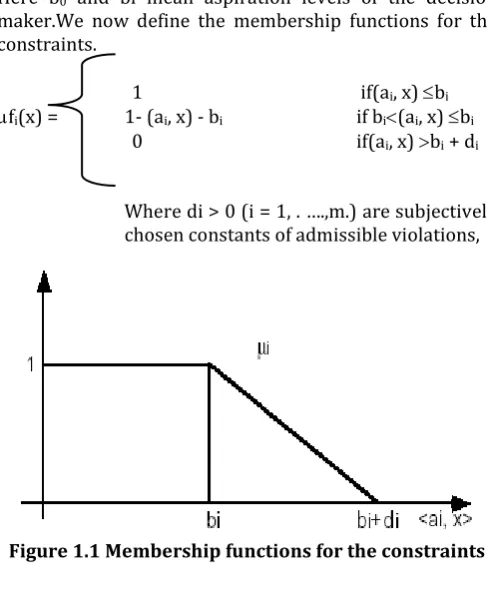
Here b0 and bi mean aspiration levels of the decision maker.We now define the membership functions for the constraints.

1 if(ai, x) bi

fi(x) = 1- (ai, x) - bi if bi(ai, x) bi

0 if(ai, x) bi + di

[image:2.595.310.554.189.489.2]

Where di > 0 (i = 1, . ….,m.) are subjectively chosen constants of admissible violations,

Figure 1.1 Membership functions for the constraints

µfi(x) is the degree to which x satisfies the ith_constraint, heredefine the membership functions for objective function

1 if(c, x) b0

fi(x) = 1-(c,x)–b0 ifb0(c,x)≤b0+d0 0 if (c, x) b0 + d0

(3)

Page 467

Figure1. 2 Membership functions of the objective function

µ0(x) is the degree to which xsatisfies the fuzzy goal function

The fuzzy decisionis defined by Bellman and Zadeh’s (1970) principle as

D (x) = min {µ0(x), µ1(x), . . ., µm(x)}

Where x can be any element of the n dimensional space, because any element has a degree of feasibility, which is between zero and one.

An optimal solution to the fuzzy LP is determined from the relationship

D (x*) = max D (x). xRn

(1) Simple Additive Model

If the criterions are quantifiable, equally important and expressed as functions of the decision variables, the Simple additive model is used to solve MODM problems Burnwal et al. (1996).

This is stated as

Find x  S, which maximizes G (g) = g1 (x) + g2 (x)+---+ gk (x)

If some or all the criterion are not quantifiable (qualitative) then with each qualitative criterion gi (x) a value function Vi (gi) is associated in terms of the decision variables.

In such cases, the model can be stated as Find x  S, which maximizes

G(g) = V1 (g1) + V2 (g2) +---+ Vk (gk)

In discrete set of action case, usually each action x  S together with its pay-off g1 (x) , g2 (x),---, gk (x) or V1 (g1) , V2 (g2) ,---, Vk (gk) is given.

(2) Weighted Additive models

In many cases all the objectives are not equally important. In such cases, weighted additive models are used in which suitable weights are assigned to reflect their relative importance. In this approach, the DM assigns weights as co-efficient of the individual terms in the simple additive value function to reflect their relative importance. These weights indicate the trade-offs between the criteria. Keeney and Raiffa (1976) and Bit, A.K. et al. (1992)have developed some weighted additive models.

The model can be stated as follows: Find x  S, which maximizes k

V (g) =  wi (x) gi (x)

or

V (g) =  wi (x) Vi (gi)

Where wi 0,  i are suitable weights to be assigned to criteria gi (x) or the associated value functions Vi (gi) satisfying the relation

k

 wi (x) =1 i =1

2. PROBLEM IDENTIFICATION

Assume that a distribution centre seeks to determine the transportation plan of a homogeneous commodity from m-source to n- destinations. Each m-source has an available supply of the commodity to distribute to various destinations and each destination has a forecast demand of the commodity to be received from the sources. The TPD proposed herein attempts to determine optimum volumes to be transported from each source to each destination to simultaneously minimize the total production cost and total delivery time. The TPD problems proposed on developing an interactive i-FMOLP model for optimizing the transportation plan in fuzzy environment.

Objective function

Practical TPD problems typically minimized the total production cost, total transportation cost and total delivery time. Accordingly two objective functions were simultaneously considered in developing the proposed MOLP , as follows:-

 Minimization total production and transportation costs

(4)

Page 468

 Minimize total delivery time

(2) Where

=total production and transportation cost($) = total delivery time(hours)

= units transported from source i to destination j = production cost/unit

= transportation cost/unit = transportation time/unit

‘=’ refers to the fuzzification of the aspiration levels.

Constraints

 Constraints on the total supply available foe each source i

= i= 1,2,………m (3)  Constraints on the total demand available foe each

source j

= ,i=1,2,………n (4)  Non-negativity constraints on decision variables

≥0, i=1,2…..m, j=1,2……n (5)

= denotes the total supply available of source i units = total demand of destination j units

MOLP model described above has a feasible solution only if the total supply available at all sources just equals the total demand required at all destinations.

3.METHODOLOGY

3.1 Linear Membership Function

The corresponding linear membership function for each fuzzy objective function is defined by:-

Where and are the lower and upper bounds. The linear membership function can be determined by requiring the DM to select the objective values interval

[ ].

In practical situation, a possible interval for imprecise objective values can be estimated based on the experience and knowledge of DM or experts, and there equivalent membership values of the DM in the interval [0,1]. Let X is a nonempty set. A fuzzy set ‘A’ of set X is defined by the following set of pairs

A}

Where

Is a mapping called the membership function of A and A(x) is the degree of membership of x in A

Thus “ a fuzzy set is a set of pair consisting of the particular elements of the universe and their membership grades.”

3.2 Multi Objective Transportation Planning Decision Using Additive Operator

Model formulation

A generalized linear model for MOTPD problem having ‘k’ objective function in ‘n’ variables subject to ‘m’ constraints can be stated as:

Optimize Subject to

X={ }≥0

Where (x) denote various cost and (x) are

various constraints.

Actually the increase/decrease in any one of the objective functions will affect the others. In MOTPD problem, the concept of an overall global optimal solution depends on the decision maker’s preference.

Assigning aspiration level vector p= ……….. to the ‘k’ objectives Which give rise to the following problem known as MOTPD. Determine X

Subject to (x) ≤ or ≥ , i= 1,2…………..k (x) ≤ or ≥ , j= 1,2………...m

In real situation all goals are not rigid. Some times some goals may be fuzzy or some rigid. Therefore it is more realistic to assign fuzzy goals by allowing some flexibility in the right hand side of some goals and some constraints. The model cannot be solved in the present form. Therefore we defuzzify this model with the help of linear membership function using the concept of fuzzy set theory.

The linear membership function corresponding to fuzzy goal may be defined as:

U1= i= 1,2………..l

U2= j= 1,2………r

3.3 Simple Additive/Compensatory Model

(5)

Page 469

Maximize the overall achievement function:

Max +

Subject to

+ =

x≥0

3.4 Normalized Weight Additive Model

In real life all objectives are not of same importance i.e. they are of varying utilities so the normalized weight may be assigned to the membership function for determining the overall achievement function V(U). The weighted additive model reflects that goals and or constraints are of varying importance. This model is widely used in multi objective programming to reflect the relative importance of goals and or constraints. Priority refers to the case when the criteria are ordered according to importance and unless the higher level criteria is taken into consideration, the next one does not come into play.

Therefore the normalized weighted additive model of MOTPD problems is stated as:

Max +

Subject to

+ =

x≥0

4. RESULTS & DISCUSSION

[image:5.595.40.565.411.768.2]

4.1 Data Discription

Table-4.1Summarized data

Source(i)

Destination(j)

Supply( )

E F G H I

A

($/hours) 18

B 22

C 14

Demand(

) 16 10 14 8 6 54

Supplies ,

Demands ,

Production cost/unit $ 10, 8, 4 respectively

Total supply available at all sources just equals the total demand required at all destinations.

4.2 SOLUTION PROCEDURE

Formulate the original fuzzy MOLP model for the transportation planning decision problems according to equation 1 to 5.

Objective function MIN(Z1)

18X11+20X12+26X13+24X14+35X15+17X21+20X22+23X 23+28X24+40X25+16X31+20X32+24X33+14X34+34X35

SUBJECT TO

X11+X12+X13+X14+X15=18 X21+X22+X23+X24+X25=22 X31+X32+X33+X34+X35=14 X14+X24+X34=8

X15+X25+X35=6 X11>=0

END469

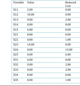
Global optimal solution found.

[image:5.595.286.556.471.762.2]

Objective value: 1112.000 Infeasibilities: 0.000000 Total solver iterations: 7

Table 4.2 Total Solver Iterations

Variable Value Reduced

Cost

X11 2.00 0.00

X12 10.00 0.00

X13 0.00 2.00

X14 0.00 8.00

X15 6.00 0.00

X21 8.00 0.00

X22 0.00 1.00

X23 14.00 0.00

X24 0.00 13.00

X25 0.00 6.00

X31 6.00 0.00

X32 0.00 2.00

X33 0.00 2.00

X34 8.00 0.00

(6)

Page 470

Objective function MIN(Z2)

4X11+5X12+8X13+12X14+30X15+10X21+10X22+12X23+ 16X24+28X25+12X31+14X32+18X33+6X34+26X35 SUBJECT TO

X12+X22+X32=10 X13+X23+X33=14 X14+X24+X34=8 X15+X25+X35=6 X11>=0

END

Global optimal solution found.

Objective value: 526.0000 Infeasibilities: 0.000000 Total solver iterations: 8

SIMPLE ADDITIVE/ COMPENSATORY MEDEL The fuzzy version of the above problem can be set as: Determine Z

Subject to Z1(X) ≤ 1112 Z2(X) ≤ 526

Now the problem is defuzzified as follows:

The linear membership functions corresponding to these fuzzy goals are defined

As follows: U1 = U2 =

Α1=90 , β1=70 and V is overall achievement The crisp model of this model is stated as: MAX U1+U2

SUBJECT TO

90U1+18X11+20X12+26X13+24X14+35X15+17X21+20X 22+23X23+28X24+40X25+16X31+20X32+24X33+14X34+ 34X35=1130

70U2+4X11+5X12+8X13+12X14+30X15+10X21+10X22+ 12X23+16X24+28X25+12X31+14X32+18X33+6X34+26X3 5=530

X12+X22+X32=10 X13+X23+X33=14 X14+X24+X34=8 X15+X25+X35=6 X11>=0

END

This problem is solved using the proposed model. On running the program on LINDO/LINGO software the results obtained are as follows:

Z1= =$1111.38, (total production and transportation cost) Z2= 491.27 hours (total delivery time)

Initially the production cost Z1= $1112. Solving the same problem using proposed compensatory model we get Z1= $1111.38. Delivery time is also reduced from 526 hours to 491.27 hours. This shows that since this problems is of cost minimization transportation cost as well as the delivery time is also decreasing here. This is due to considering inexactness or fuzziness in parameter.

The result of the process shows that when we change in normalized weight then we get production cost and operating cost Z1= $1093.38 and operating time Z2= 463.91hours at w1=.8 & w2= .6 which one is less than the earlier values of Z1 & Z2. If we change in aspiration level then again the value of Z1 & Z2 is increased. When we change in normalized weight and aspiration level both then we get the value of Z1 & Z2 is $1094.35 and 501.65hours respectively. finally if we change in all means change in normalized weight and aspiration level and tolerance limit then we get production cost and operating cost Z1 is $1084.27 which is minimum and operating time 505.63 hours is obtained. A set of numerous compromising solution for the problem are obtained from which decision maker may use one for his best use.

5. CONCLUSION

Fuzzy linear model for multi-objective transportation planning decision allows flexibility in constraints, which is not possible with any deterministic model. The deterministic model gives unique result i.e. total production and transportation cost Z1= $1112 and delivery time Z2= 526 hours. Solving the same problem using the proposed fuzzy model we get different value of Z1 and Z2 by changing normalized weight, aspiration level and both respectively as shown in table 4. A set of numerous compromising solution for the problem are obtained from which decision maker may use one for his best use.

REFERENCES

[1]. L. H. Chen and F.C.Tsai (2006) , fuzzy goal programming with different important and priorities, European journal of operational research, vol. 133, pp. 548-556

(7)

Page 471

[3]. S.Chanas and D. Kuchta(1996) , A concept of the optimal solution of the transportation problem with fuzzy cost coefficient, vol. 82, pp. 299-305

[4]. A.K. Bit, M.P. Biswal and S.S. Alam (1992) fuzzy programming approach to multi criteria decision making transportation problem,Fuzzy set and system , vol. 50, pp. 35-41

[5]. Tien-Fu Liang (2009) Applying interactive fuzzy

multi objective linear programming to

transportation planning decision. Vol. 27, pp. 107-126

[6]. J. Current and M.Marish (1993) Multi-objective transportation network design and routing problems, European journal of operations research, vol.65, pp. 4-19

[7]. Y.P.Aneja and K.P.K. Nair (1979), Bicriteria transportation problems , Management science, vol. 25, pp. 73-78

[8]. Chanas, S., Kuchta, D., (1998). Fuzzy integer transportation problem. Fuzzy Sets and Systems 98, 291–298.

[9]. Abd El-Wahed W.F., (2001). A multi-objective transportation problem under fuzziness. Fuzzy Sets and Systems,117: 27-33.

[10]. Abd El-Wahed W.F., S.M. Lee, (2008). Interactive fuzzy goal programming for multi-objective transportation problems. Omega, 34(2): 158-166. [11]. Arsham, H., A.B. Khan, (1989). A simplex type

algorithm for general transportation problems: An alternative to stepping-ston, Journal of Operations Research Society,40: 581-590.

[12]. Bellman, R.E. and L.A. zadeh, (1970). Decision making in fuzzy enviouroment, management Science, 17: 141-164.

[13]. Bit, A.K., M.P. S.S. Biswal, (1992). Alam Fuzzy programming approach to multi-criteria decision making transportation problem. Fuzzy Sets and Systems, 50(2): 135-141.

[14]. Chanas, S., D. Kutcha, (1996). A concept of optimal solution of transportation problem with fuzzy cost coeffiencts,fuzzy sets and systems, 82: 299- 308. [15]. Chanas, S., D. Kutcha, (1998). fuzzy integer

Multi Objective Programming For Transportation Planning Decision

Page 465