r a ti n g s u si n g m a c h i n e l e a r ni n g
a n d c o n v e n ti o n al t e c h ni q u e s
Ab d o u , HA H, Ab d all a h , W M, M ul k e e n , J, N ti m , CG a n d Wa n g , Y
1 0 . 2 1 5 1 1 /i mfi. 1 4( 4). 2 0 1 7 . 1 6
T i t l e
P r e d i c ti o n of fi n a n ci al s t r e n g t h r a ti n g s u si n g m a c h i n e
l e a r n i n g a n d c o n v e n ti o n al t e c h n i q u e s
A u t h o r s
Ab d o u , HA H , Ab d all a h , W M, M u lk e e n , J, N t i m , CG a n d
Wa n g , Y
Typ e
Ar ticl e
U RL
T hi s v e r si o n is a v ail a bl e a t :
h t t p :// u sir. s alfo r d . a c . u k /i d/ e p ri n t/ 4 4 9 3 3 /
P u b l i s h e d D a t e
2 0 1 7
U S IR is a d i gi t al c oll e c ti o n of t h e r e s e a r c h o u t p u t of t h e U n iv e r si ty of S alfo r d .
W h e r e c o p y ri g h t p e r m i t s , f ull t e x t m a t e r i al h el d i n t h e r e p o si t o r y is m a d e
f r e ely a v ail a bl e o nli n e a n d c a n b e r e a d , d o w nl o a d e d a n d c o pi e d fo r n o
n-c o m m e r n-ci al p r iv a t e s t u d y o r r e s e a r n-c h p u r p o s e s . Pl e a s e n-c h e n-c k t h e m a n u s n-c ri p t
fo r a n y f u r t h e r c o p y ri g h t r e s t r i c ti o n s .
Abstract
Financial strength ratings (FSRs) have become more significant particularly since the recent financial crisis of 2007–2009 where rating agencies failed to forecast defaults and the downgrade of some banks. The aim of this paper is to predict Capital Intelligence banks’ financial strength ratings (FSRs) group membership using machine learning and conventional techniques. Here the authors use five different statistical techniques, namely CHAID, CART, multilayer-perceptron neural networks, discriminant analysis and logistic regression. They also use three different evaluation criteria namely average correct classification rate, misclassification cost and gains charts. The data are collect-ed from Bankscope database for the Middle Eastern commercial banks by reference to the first decade of the 21st century. The findings show that when predicting bank FSRs during the period 2007–2009, discriminant analysis is surprisingly superior to all other techniques used in this paper. When only machine learning techniques are used, CHAID outperform other techniques. In addition, the findings highlight that when a random sample is used to predict bank FSRs, CART outperform all other techniques. The evaluation criteria have confirmed the findings and both CART and discriminant analysis are superior to other techniques in predicting bank FSRs. This has implica-tions for Middle Eastern banks, as the authors would suggest that improving their bank FSR can improve their presence in the market.
Hussein A. Abdou (UK), Wael M. Abdallah (Egypt), James Mulkeen (UK),
Collins G. Ntim (UK), Yan Wang (UK)
BUSINESS PERSPECTIVES
LLC “СPС “Business Perspectives” Hryhorii Skovoroda lane, 10, Sumy, 40022, Ukraine
www.businessperspectives.org
Prediction of financial
strength ratings using
machine learning and
conventional techniques
Received on: 1st of November, 2017
Accepted on: 19th of December, 2017
INTRODUCTION
A bank’s financial strength, its risk profile, soundness and financial stability are assessed by Capital Intelligence (CI) banks’ financial strength ratings (FSRs). This incorporates factors within its internal and external environment. CI implements a specialized approach, including some qualitative and quantitative factors, in assessing a bank’s stability and thus assigning the appropriate banks’ FSR. This is achieved by grouping factors into the following six broad categories: ownership and governance; operating environment; management and strategies; franchise value; risk profile and financial profile. Internally, CI assesses a bank’s governance and specifically the extent to which there is a division between ownership and the management of its oper-ations. Bridging the gap between a bank’s internal and external envi-ronment, CI examines a bank’s domestic market share as reflected in its assets and its potential future earnings (see, for example, Abdallah, 2013). As such, CI assesses these factors and generates a bank’s FSRs.
In the Middle East region, financial stability and soundness are entirely affected by the host country’s banking system. This is mainly due to the absence of the capital markets’ role in resource allocation and thus FSR is
© Hussein A. Abdou, Wael M. Abdallah, James Mulkeen, Collins G. Ntim, Yan Wang, 2017
Hussein A. Abdou, Ph.D., Professor of Banking & Finance; Department of Accounting, Finance and Banking, Faculty of Business and Law, Manchester Metropolitan University, Manchester, UK; and Management Department, Faculty of Commerce, Mansoura University, Mansoura, Egypt.
Wael M. Abdallah, Ph.D., Assistant Professor of Finance, Department of Finance, Misr International University, Egypt.
James Mulkeen, Ph.D., Reader in Leadership & Management, Saloford Business School, University of Salford, UK.
Collins G. Ntim, Ph.D., Professor of Accounting, Department of Accounting, School of Management, University of Southampton, UK. Yan Wang, Ph.D., Senior Lecturer in Accounting and Finance, Department of Accounting and Finance, Faculty of Business & Law, De Montfort University, UK.
This is an Open Access article, distributed under the terms of the
Creative Commons Attribution-Non-Commercial 4.0 International license, which permits re-use, distribution, and reproduction, provided the materials aren’t used for commercial purposes and the original work is properly cited.
FSR group membership, Capital Intelligence, machine learning techniques, conventional techniques, Middle East
Keywords
seen as an important indicator of the banking systems soundness and stability. As such, a bank’s FSR is con-sidered as an important indicator for various stakeholders in assessing the bank’s FSRs. This is particularly important due to deficiencies in legal and regulatory systems and lack of transparency within banking sec-tors and financial markets (Abdallah, 2013). The difficulty in developing accurate rating systems for banks as opposed to countries is reflected in the relative inability of rating agencies to agree a universal rating sys-tem. A strong bank FSR assists a bank in accessing capital markets with more favorable conditions, as well as positively affecting its operations and performance (Hammer et al., 2012). In addition, these rating agencies have been accused of being liable for the ‘housing bubble’ and consequently financial crash of 2007–2008 (Diomande et al., 2009).
In the literature, less attention is paid to the Middle East region due to a number of factors that appear to be influential in this respect. First, governments are the main source for Middle Eastern banks’ equity financing. Second, the need to assess a bank’s creditworthiness is reduced where the bank is government-owned, be-cause the government uses their banks to finance economic activities. This may be-cause a disconnect between the bank’s FSRs and its capital structure. Third, the underdeveloped legal and regulatory system has resulted in a weak system to monitor capital risk in Middle Eastern countries (see of commercial banks in the Middle East that is 64 out of 135, as per Bankscope database 2011, are rated. The development of stock markets in the Middle East has encouraged the operation of foreign rated banks within the region and this, in turn, has resulted in improving the competitiveness and performance of non-rated banks. This raises banks’ interests in obtaining adequate FSRs.
The motivation of our investigation is to evaluate and rank the predictive capabilities of machine learning and conventional techniques using different decision criterion namely error rates, misclassification costs and gains charts for different sample sizes. Due to scarcity of studies related to banks’ FSR under Capital Intelligence (CI), the objective of this paper is to determine whether Middle Eastern bank’s financial and non-financial indicators can be used to predict their FSR group membership. The novelty of this paper is to apply machine learning and conventional techniques to predict a bank’s CI FSR by distinguishing high rat-ings from low rating using financial and non-financial indicators. We use banks’ FSRs issued by CI rating agency for Middle Eastern commercial banks1 in the first decade of the 21st century2, which is ignored in the
literature. There is no empirical study, which, to the best of our knowledge, uses non-financial indicators to capture the effect of country specific differences, with other firm level characteristics, to determine whether they are able to distinguish high from low CI FRSs. The remainder of this paper is organized as follows: sec-tion 1 reviews literature; secsec-tion 2 outlines the research methodology and data collecsec-tion; secsec-tion 3 provides a discussion of the empirical findings and compares results of different bank FSR group membership models; and the last section concludes the paper and highlights areas for future research.
1 CI is more specialized in rating banks in the Middle East region than Fitch and Moody’s. According to Bankscope database as at January 2011, CI assigns bank FSRs for 64 commercial banks in the Middle East region compared to Fitch and Moody’s who assign bank ratings for only 50 and 48 commercial banks, respectively. S&Ps has no publically available equivalent individual bank ratings in the period 2001–2009.
2 The reason to choose the first decade of the 21st century is to avoid any potential effect of the Arab spring which commenced in 2010 and the huge missing data due to this phenomenon. However, it is part of our future research plan to investigate the effect of the Arab spring on bank ratings in the Middle East.
1.
REVIEW OF RELEVANT
LITERATURE
As early as the 1960s, there were studies that focused on forecasting business events and classifying com-panies into two or more separate groups. Many re-searchers have applied different conventional and advanced statistical techniques to build
ratings for developed economies (see, for example, Poon et al., 1999; Poon & Firth, 2005; Hammer et al., 2012; Beisland et al., 2014), but not the relationship between financial/non-financial factors and bank ratings. Unsurprisingly, less attention has been paid to developing economies and in particular to the Middle East region.
Various statistical machine learning techniques are used in predicting bank rating (see for example, Chen, 2012; Chen & Cheng, 2013). CART algorithms has been employed in a number of situations. For exam-ple, to predict bankruptcy (Chandra et al., 2009; Li et al., 2010); to develop credit scoring models for assess-ing the credit risk of bank customers (Lee et al., 2006; Kao et al., 2012); to develop early warning models to assess the soundness of individual banks (Loannidis et al., 2010); and to predict bank performance (Ravi et al., 2008). Many studies into early warning system models for financial risk (Koyuncugil & Ozgulbas, 2012) and for developing credit scoring models for assessing bank customers credit risk (Thomas et al., 2002; Bijak & Thomas, 2012) have utilized CHAID algorithms. To the best of our knowledge, this is the first paper that uses both CART and CHAID algo-rithms to predict Middle Eastern commercial banks’ FSRs.
Based on human brains, neural networks are non-parametric techniques and computational meth-ods that are used to identify significant patterns or structures in data which are then used to predict future phenomena. Neural networks have been ap-plied in various financial studies such as: to predict bankruptcy of banks (Kumar & Ravi, 2007; Ravi & Pramodh, 2008; Zhao et al., 2009; Loannidis et al., 2010); to predict bankruptcy of firms (Chandra et al., 2009; Falavigna, 2012); to evaluate banks’ creditwor-thiness (see, for example, Huang et al., 2004), and to predict banks’ financial strength rating (Poon et al., 1999; Pasiouras et al., 2007; Hammer et al., 2012).
Altman (1971) introduced DA z-score model that discriminates bankrupt from non-bankrupt firms. In finance literature Altman and Sametz (1977), Canbas et al. (2005), Li et al. (2010) apply many forms of the DA to predict corporate and bank failure and assessing financial distresses. In addi-tion, DA has been employed by Lee et al. (2006), Abdou et al. (2008), Abdou (2009a), Akkoc (2012)
in building credit scoring models. In the field of
banking DA and hybrid techniques are used in rating predictions (see, for example, Chen, 2012; Chen & Cheng, 2013).
In the literature on finance, LR is a widely-used technique among practitioners in predicting corporate and bank failure (Kolari et al., 2002; Canbas et al., 2005; Zhao et al., 2009; Li et al., 2010; Abdou et al., 2016); in predicting credit rat-ings (Oelerich & Poddig, 2006; Kim & Ahn, 2012); as well as in building credit scoring models (Lee et al., 2006; Abdou et al., 2008; Abdou, 2009a; Akkoc, 2012; Abdou et al., 2016). Finally, the LR model is employed by Poon et al. (1999), Hammer et al. (2012) to predict bank financial strength rat-ing. Predicting both Moody’s BFSRs (see Poon et al., 1999) and Fitch FBRs (Pasiouras et al., 2007; Hammer et al., 2012) have been the focus of the majority of previous studies. It is notable that there is no previous study focused upon CI FSRs (see, for example, Abdallah, 2013). Consequently, the focus of our investigation is to bridge this gap by using both machine learning and conventional techniques to predict banks’ CI FSRs group mem-bership in Middle Eastern commercial banks.
2.
RESEARCH METHODOLOGY
From Figure 1, it can be observed that the auto-clas-sifier node ranks the two decision trees techniques namely CHAID, with an overall accuracy of 96.30%, and CART, with an overall accuracy of 95.44%, as first and second. These two techniques are followed by MLP NN with an overall accuracy of 94.02%. In addition, there is a role for DA as one of the conven-tional techniques with an overall accuracy of 93.16%, which is comparable with the machine learning techniques. However, the auto-classifier node ranks LR far below the other four techniques with an over-all accuracy of only 73.5%. Therefore, it can be sug-gested that CHAID, CART, MLP NN and DA could perform better compared to LR in predicting Middle Eastern commercial banks’ FSRs. Finally, four differ-ent evaluation criteria namely average correct clas-sification (ACC) rate, error rates, estimated misclas-sification cost (EMC) and gains charts are used to evaluate the predictive capabilities of these statistical modeling techniques.
2.1. Statistical modelling techniques
2.1.1. Bank FSR machine learning techniques
CHAID
The Chi-squared Automatic Interaction Detector (CHAID) is a statistical technique used to assess the relationship between a target variable and
a series of predictor variables (see, for example, Koyuncugil & Ozgulbas, 2012; Abdallah, 2013). A CHAID model divides the data into mutually ex-clusive and exhaustive sub-sets that best describe the target variable and predict the interaction be-tween predictor variables (Bijak & Thomas, 2012; Abdallah, 2013). For categorical dependent vari-ables, Chi-squared is used as a measurement lev-el, whilst for continuous dependent variables the F-test is used instead (SPSSInc, 2012). In building our CHAID models, we use Pearson Chi-squared statistics which are calculated using both observed expected cell frequencies with the p-value being based on the calculated statistics.
The Pearson Chi-squared statistic is calculated as follows (see, for example, PASW, 2012, p. 77; Abdallah, 2013, modified):
(
)
2 21 1
,
J I
ij ij
j i ij
n ˆ
X ˆv
v = =
=
∑∑
− (1)where ij n
(
n n)
nn f I x=
∑
⋅ ⋅ = ∧i y = j refers to theactual cell frequency; ˆvij refers to the expected
cell frequency for cell ( xn =i, yn= j ) from the
independence model; br 2 2 d
b= ⋅( x >X ) refers to the calculation of the corresponding p-value,
where 2 d
x follows a Chi-squared distribution with
(
1) (
1)
[image:5.595.135.534.92.305.2]d = J – ⋅ I – df .
CART
The Classification and Regression Trees (CART) is a classification non-parametric statistical model, which can use a binary decision tree-based pro-cedure. It can be simultaneously applied to both categorical and continuous data based on a set of ‘if-then’ rules. It automatically separates com-plex databases for separating significant patterns and relationships (Ravi et al., 2008; Chandra et al., 2009; Abdallah, 2013). CART methodology can be divided into three phases: first, the construction of a maximum tree (tree-growing process); second, the selection of the right-sized tree (pruning pro-cess); third, the classification of the new data us-ing the constructed tree. Gini index is used as part of the process, and the model repeats the splitting process until either the homogeneity criterion is reached or other stopping criteria are fulfilled. The Gini index uses the following impurity function
( )
g t at a node t in CART tree (PASW, 2012, p. 63; Abdallah, 2013; Abdou et al., 2016, modified):
( )
( ) ( )
,j i
G r b j r b i r ≠
=
∑
⋅ (2)where i and j are categories of the independent predictor variable, and
( )
b j,r( )
( )
,b j r
b r
= (3)
( )
( )
j( )
,j
j N r b j r
N
π ⋅
= (4)
( )
(
, ,)
j
b r =
∑
b j r (5)where π
( )
j refers to the prior probability value for category j; N rj( )
refers to the number of records in category j of node r, and Nj refers to the num-ber of records of category j in the root node. The Gini index enhances splitting during tree growth process. As such, N rj( )
and Nj are only calculat-ed, respectively, from the records on node r and the root node with valid values for the split-predictor.Then, ‘the pruning process’ improves generaliza-tion to avoid over-fitting by applying two pruning algorithms. First is the optimization by number of points in each node pruning algorithm which im-plies that the splitting is stopped when the number
of observation in the node is the pdefined re-quired minimum number of observations. Second is the cross-validation pruning algorithm, which establishes an optimal proportion between the misclassification error and the complexity of the tree. As such, the focus of the cross-validation pruning algorithm process is to use the minimal cost-complexity function to minimize both mis-classification risk and the complexity of the tree in order to obtain an optimal tree as follows (see, for example, PASW, 2012, p. 67; Abdallah, 2013):
R C R C C , (6)
where R C
( )
refers to the misclassification risk of tree C; C refers to the number of terminal nodes for tree C; and α refers to the complexity cost per terminal node for the tree. Finally, following the construction of right-size tree with the low-est cross-validated rate, the outcome of the third phase process is to classify the new data. As such, based on a set of rules, each new observation is as-signed to a class or response value that fits with one of the terminal nodes of the tree.Multilayer-Perceptron
Neural Networks
Multilayer-Perceptron Neural Network (MLP NN) enables the analysis of complex relationships be-tween different variables and consists of layers of interconnected nodes between the input layer and the output layer. As part of the network nomen-clature, predicted outputs are generated and com-pared with actual outputs in order to calculate an error function. The network repeats the process un-til the either of the number of iterations is reached or the error function is almost zero.
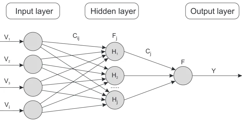
An architecture of MLP NN is shown in Figure 2. This consists of an input layer with a number of neurons with their dendrites for input predic-tor variables
(
V V1, ;2…Vi)
the hidden layer with a number of neurons( );
L and the output layer Y. The statistical formula of MLP NN with onehid-den layer is as follows (Abdallah, 2013, modified):
1 1
,
J i
j j ij i
j i
Y F C F C V
= =
= ⋅ ⋅ ⋅
∑
∑
(7)where Y refers to the network output; F refers
connec-tion weights from L to Y F, j refers to the
trans-fer function for L C, ij refers to the connection
weights from
(
V V1, 2…Vi)
to L, and Vi refersto the input predictor variable (see for example, Abdou, et al., 2014; Abdallah, 2013; Brown & Mues, 2012, modified).
2.1.2. Conventional techniques
Discriminant analysis
Discriminant analysis (DA) is a classification tech-nique widely used to develop a Z-score model to discriminate between two or more groups of ob-servations (Abdou et al., 2008). DA predicts and classifies problems where the nature of the depen-dent variable is binary, for example, high versus low risk, high versus low FSRs etc. The formula used in DA is as follows:
1 1 ,2 2 n n
Z = + ⋅ +α a V a V⋅ + … + a V⋅ (8)
where Z refers to the discriminant outcome score which reflects group differences; α refers to the intercept; a a1, , ..., 2 an are the discriminant
coef-ficients; and V V1, 2…Vn refer to the independent
variables (see, for example, Abdou et al., 2008; Abdallah, 2013).
Logistic regression
Logistic regression (LR) is a multivariate statisti-cal technique used for prediction purposes in cas-es where the dependent variable is dichotomous. Binomial probability is used to develop a logit function from conventional linear regression. LR formula is as follows (see, for example, Abdallah, 2013; Abdou et al., 2016):
1 1 2 2
1b n n,
Log V V V
b α β ⋅ β β
= + + +…+
⋅
− ⋅
(9)
where b refers to the output probability;
α
refers to the intercept of the equation; and β β1, ... 2 βnrefer to the coefficients in the linear combination of the independent variables V V1, 2…Vn.
2.2. Data collection, variables
and sampling
2.2.1. Data collection
[image:7.595.84.500.84.294.2]In order to develop the proposed bank FSR group membership models, we use 64 commer-cial banks rated by Capital Intelligence (CI) out of a total number of 135 Middle Eastern banks in our original sample. As the vast majority of
Figure 2. MLP feed-forward NN architecture (one hidden layer)
Input layer
Hidden layer
Output layer
V1
V2
V3
Vi
Cij
Cj Fj
F
Y H1
... H2
Hj
banks in the Middle Eastern region are com-mercial banks, we then focus on this group of banks to avoid any potential comparison prob-lems between different types of banks and for homogeneity across different countries included in our final sample. We use data from 10 Middle Eastern countries3, as shown in Table 1. Our
da-ta are collected from Bankscope dada-tabase by
3 Israel, Palestinian Territory, Iraq and Syrian Arab Republic are excluded from the sample, because they do not have commercial banks rated by CI. Iran is also excluded from the sample as all Iranian banks are classified as Islamic banks.
reference to the first decade of the 21st century,
i.e., 2001–2009.
[image:8.595.71.525.488.725.2]Descriptive statistics for each of the 10 countries’ banks based on their natural log of total assets ($) are shown in Table 1. Clearly, banks in Bahrain, Kuwait and Saudi Arabia are larger in size than other countries in our final sample. By contract,
Table 1. Descriptive statistics for banks, by country and whether rated by CI based on size (ln total assets)
Country commercial No. of
active banks
No. of banks with
CI’s FSR % of banks rated by CI, % Mean size deviation Standard
Egypt 24 6 25 8.809 0.855
Bahrain 10 4 40 9.422 0.819
Kuwait 6 6 100 9.231 0.598
Jordan 11 7 63.6 7.433 1.296
Qatar 8 4 50 8.547 1.146
Lebanon 38 6 15.7 8.688 0.708
Saudi Arabia 9 9 100 9.672 0.815
United Arab Emirates 18 15 83.3 8.248 1.316
Oman 6 5 83.3 7.810 0.708
Yemen 5 2 40 5.832 0.554
Total 135 64 47.4 8.521 1.308
Note: Size is measured by ln total assets. The initial sample consists of 135 active commercial banks (of which 64 are rated by CI) covering 10 countries from the Middle East region: Egypt, Bahrain, Kuwait, Jordan, Qatar, Lebanon, Saudi Arabia, United Arab Emirates, Oman and Yemen. The data are extracted from Bankscope for 9 years from 2001 to 2009 inclusive.
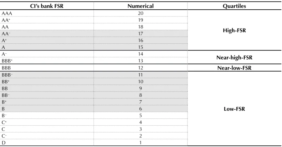
Table 2. A synopsis of CI bank FSRs numerical ratings and rating categories
CI’s bank FSR Numerical Quartiles
AAA 20
High-FSR
AA+ 19
AA 18
AA– 17
A+ 16
A 15
A– 14
Near-high-FSR
BBB+ 13
BBB 12 Near-low-FSR
BBB– 11
Low-FSR
BB+ 10
BB 9
BB– 8
B+ 7
B 6
B– 5
C+ 4
C 3
C– 2
D 1
banks in Yemen tend to be smaller in size when compared to other banks in other countries in the sample. In addition, banks in Egypt, Qatar, Lebanon and United Arab Emirates have a similar average size, as do banks in Jordan and Oman.
2.2.2. Dependent variable
As shown in Table 2, we rank CI banks’ FSR us-ing a scale from 1 up to 20; where 1 refers to the lowest FSR rating category (D) and 20 refers to the highest FSR rating category (AAA) (see, for exam-ple, Poon et al., 2009). As also shown in Table 2, the highest FSR rating category for banks in the Middle East region in our sample is AA– (17) and
the lowest FSR rating category is B (6). We use a simple weighted average to divide the data into four quartiles. Then, we use the highest quartile (15 to 17) versus the lowest quartile (6 to 11) as our dependent categorical variable4.
2.2.3. Independent variable
Selected independent variables for the proposed models are reduced to 17 financial and non-finan-cial variables5.
Financial variables
We use different financial ratios under the follow-ing categories: asset quality, capital adequacy, prof-itability, credit risk and liquidity, following CI rat-ing agency, to predict Middle Eastern banks’ FSR group membership, as shown in the Appendix.
Non-financial variables
In this paper, authors examine non-financial vari-ables that may improve a models predictive capa-bility in terms of a bank’s FSR group membership. The following three non-financial variables are used: first, we use size as a dummy variable which is measured by ln total assets. To reflect qualitative characteristics such as product diversification and geographic location, we classify banks’ size into small, medium and large. Second, we use a dum-my variable for the effect of time. Third, we use CI’s country sovereign risk ratings (SR) to reflect
4 Low-FSR banks are 179 observations while high-FSR banks are 172 observations.
5 The issue of multicollinearity is addressed by examining the Variance Inflation Factor (VIF) scores. The regression analysis is run for number of times to trace the variables associated with VIF scores > 5 (Abdallah, 2013).
differences in the implemented regulatory systems across countries. In calculating SR, the following macroeconomic factors are considered: inflation, taxation, exchange rates, infra-structure, employ-ment rate, size and the growth of economy and regulations. Sovereign ratings reflects the prob-ability that a government may default in meeting their obligations (see, for example, Abdallah, 2013; Laere et al., 2012). Correlation between our final-ly selected variables indicates no serious correla-tion (i.e., > 0.60) found amongst these variables, as shown in the following section.
We divided the data-set into two samples. Sample1 (we use 2001–2006 observations as a training sub-sample1, 235 observations; and 2007–2009 obser-vations as a hold-out sub-sample1, 116 observa-tions). Sample2 (67% training sub-sample2, 235 observations; and 33% hold-out sub-sample2, 116 observations), which are randomly selected by the PASW@ Modeler 14 software.
3.
EMPIRICAL FINDINGS
PASW® Modeler 14, Scorto and IBM SPSS 22 soft-ware are used in this paper to build the proposed models. The descriptive statistics and detailed bank FSR group membership results for the cho-sen statistical techniques are summarized below.
3.1. Descriptive statistics
Correlation results between our predictor indica-tors including the dependent variable (high-FSR versus low-FSR), are shown in Table 3. All correla-tions between predictor indicators are within an acceptable range, i.e., < 0.60. Table 3 highlights that the highest correlation coefficient of 0.588 is between LLPTL and NIEAA. We argue that there is no multicollinearity problem between them as only correlations over 0.80 cause a serious prob-lem (see, for example, Abdou et al., 2016).
3.1.1. Financial indicators
Table 3. Correlation matrix for predictor variables
LL
PN
IR
LL
R
IL
ILG
L
TC
R
CS ENL EM NIM
NI
EA
A
RE
P
A
U
TM
E
LL
PT
L
LADS
TF
Ti
m
e
SR Size CAT
LLPNIR 1 – – – – – – – – – – – – – – – – –
LLRIL –.179** 1 – – – – – – – – – – – – – – – –
ILGL .306** –.461** 1 – – – – – – – – – – – – – – –
TCR –.144* –.003 .177** 1 – – – – – – – – – – – – – –
CS –.218** .141* –.445** .169** 1 – – – – – – – – – – – – –
ENL –.052 –.100 .195** .581** .247** 1 – – – – – – – – – – – –
EM .353** –.130* .153** –.254**–.447** –.118* 1 – – – – – – – – – – –
NIM –.270** –.058 .097 .178** .264** –.006 –.168** 1 – – – – – – – – – –
NIEAA .511** –.298** .479** –.108 –.207**–.154** .284** .227** 1 – – – – – – – – –
REP .180** .239** –.193** .125* .411** .001 –.207** .533** .077 1 – – – – – – – –
AU .391** –.090 .349** .225** –.216** –.004 .155** .290** .518** .424** 1 – – – – – – –
TME –.039 .141* –.177** .058 .147** –.001 –.135* .001 –.157** .111* –.118* 1 – – – – – –
LLPTL .548** –.236** .500** .259** –.274** .334** .364** .081 .588** .225** .469** –.126* 1 – – – – –
LADSTF .040 –.255** .360** .330** .001 .436** .007 –.095 .029 –.182** –.015 –.150** .204** 1 – – – –
Time –.002 .132* –.202**–.161** .003 –.042 .020 –.056 –.108* .040 .097 .077 –.030 –.271** 1 – – –
SR –.066 .403** –.536**–.252** .457** –.353**–.256** –.020 –.208** .324** –.337** .212** –.354**–.346** .103 1 – –
Size –.011 .415** –.505**–.345** –.107* –.274** .051 –.267**–.336** .004 –.256** .144** –.232**–.385** .405** .453** 1 –
CAT –.153** .467** –.572**–.209** .074 –.317** –.119* –.076 –.350** .160** –.391** .177** –.297**–.374** .096 .432** .523** 1
Notes: The overall sample consists of 135 active commercial banks (of which 64 banks rated by CI) covering 10 countries from Middle East region: Egypt, Bahrain, Kuwait, Jordan, Qatar, Lebanon, Saudi Arabia, United Arab Emirates, Oman and Yemen. The data are extracted from Bankscope for the years 2001–2009 inclusive.
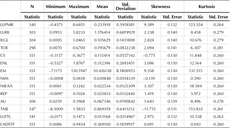
Table 4. Descriptive statistics for the 14 financial indicators
N Minimum Maximum Mean DeviationStd. Skewness Kurtosis
Statistic Statistic Statistic Statistic Statistic Statistic Std. Error Statistic Std. Error
LLPNIR 340 –0.4375 8.6851 0.251918 0.5918581 9.389 0.132 123.554 0.264 LLRIL 303 0.0953 5.8233 1.176414 0.6819929 2.238 0.140 8.458 0.279 ILGL 304 0.0005 1.0465 0.105629 0.1431808 2.824 0.140 10.676 0.279 TCR 298 0.0070 0.6700 0.195679 0.0832238 2.094 0.141 6.307 0.281 CS 351 –0.3137 0.3677 0.115414 0.0557142 –0.775 0.130 11.848 0.260 ENL 351 –0.5327 1.8767 0.312396 0.2693451 3.086 0.130 12.164 0.260 EM 351 –7.1175 130.1947 10.426138 8.1806933 9.358 0.130 131.515 0.260 NIM 351 –0.0008 0.0618 0.030848 0.0104339 –0.139 0.130 0.590 0.260 NIEAA 351 0.0061 0.1242 0.022534 0.0125309 3.307 0.130 18.584 0.260 REP 351 –0.0097 0.1024 0.025833 0.0132440 1.419 0.130 5.972 0.260 AU 306 0.0259 0.1968 0.067346 0.0190842 1.643 0.139 8.496 0.278 TME 347 –8.5000 1.5833 0.869359 0.6413212 –11.715 0.131 153.833 0.261 LLPTL 341 –0.0171 0.1473 0.013168 0.0214967 2.975 0.132 10.538 0.263 LADSTF 351 0.0086 0.9434 0.369100 0.1839937 0.691 0.130 0.043 0.260
[image:10.595.73.529.458.710.2]10.426 (and the highest standard deviation value of 8.181) and LLPTL has the lowest mean value of 0.013 (NIM has the lowest standard deviation val-ue of 0.010). Table 5 shows group statistics for the 14 financial predictors for both high-FSR and FSR. Again EM has the highest high-FSR and low-FSR mean values of 11.379 and 9.435, respectively
[image:11.595.72.526.101.608.2](EM also has the highest standard deviation val-ues for high-FSR and low-FSR of 9.456 and 6.621, respectively). LLPTL has the lowest high-FSR and low-FSR mean values of 0.007 and 0.019, respec-tively (NIM has the lowest standard deviation val-ue for high-FSR and low-FSR of 0.007 and 0.013, respectively).
Table 5. Group statistics for the 14 financial indicators
CAT N Mean Std. Deviation Std. Error Mean
LLPNIR High-FSR 172 0.162755 0.2880616 0.0219645
Low-FSR 168 0.343203 0.7807317 0.0602348
LLRIL High-FSR 164 1.468992 0.7288206 0.0569113
Low-FSR 139 0.831213 0.4107235 0.0348371
ILGL High-FSR 165 0.030640 0.0295505 0.0023005
Low-FSR 139 0.194644 0.1710849 0.0145112
TCR High-FSR 167 0.180305 0.0540258 0.0041806
Low-FSR 131 0.215277 0.1067987 0.0093310
CS High-FSR 172 0.119607 0.0285815 0.0021793
Low-FSR 179 0.111385 0.0727009 0.0054339
ENL High-FSR 172 0.225523 0.0640988 0.0048875
Low-FSR 179 0.395871 0.3527058 0.0263625
EM High-FSR 172 9.434960 9.4559659 0.7210106
Low-FSR 179 11.378556 6.6205101 0.4948402
NIM High-FSR 172 0.030043 0.0065669 0.0005007
Low-FSR 179 0.031621 0.0130922 0.0009786
NIEAA High-FSR 172 0.018070 0.0071052 0.0005418
Low-FSR 179 0.026825 0.0149159 0.0011149
REP High-FSR 172 0.027992 0.0078521 0.0005987
Low-FSR 179 0.023759 0.0166384 0.0012436
AU High-FSR 147 0.059595 0.0122440 0.0010099
Low-FSR 159 0.074512 0.0213763 0.0016953
TME High-FSR 172 0.983616 0.0402651 0.0030702
Low-FSR 175 0.757061 0.8892001 0.0672172
LLPTL High-FSR 172 0.006839 0.0093660 0.0007142
Low-FSR 169 0.019610 0.0276255 0.0021250
LADSTF High-FSR 172 0.298933 0.1620916 0.0123594
Low-FSR 179 0.436523 0.1788769 0.0133699
3.1.2. Non-financial indicators
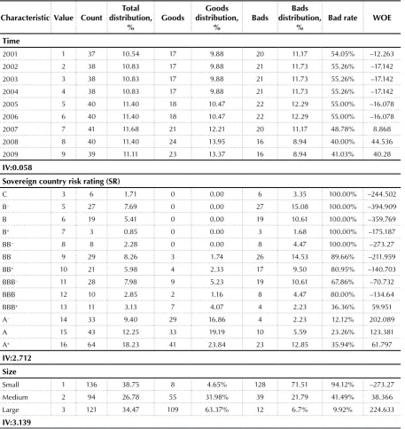
Descriptive statistics for the 3 non-financial pre-dictor indicators are shown in Table 6. As per the information value6 score, ‘Size’ is the most
in-fluential non-financial predictor with a sore of 3.139. ‘Sovereign Country Risk Rating’ (SR) with an information value score of 2.712 comes second.
6 Information value directly relates to a statistical technique called Weight of Evidence (WoE) which identifies the strength of different predictor indicators, as an alternative to Chi2. For more details the reader is referred to Abdou et al. (2016).
[image:12.595.71.529.100.585.2]Finally, ‘Time’ shows the lowest importance with information value score of 0.058. The latter value indicates that ‘Time’ has no effect on our Middle Eastern banks sample from 2001 to 2009 even during the financial crisis, i.e., 2007–2009. This implies that the effect of the financial crisis on Middle Eastern banks during this period was not evident, but it might have an effect in later years.
Table 6. Descriptive statistics for non-financial indicators
Characteristic Value Count distribution, Total
% Goods
Goods distribution,
% Bads
Bads distribution,
% Bad rate WOE
Time
2001 1 37 10.54 17 9.88 20 11.17 54.05% –12.263
2002 2 38 10.83 17 9.88 21 11.73 55.26% –17.142
2003 3 38 10.83 17 9.88 21 11.73 55.26% –17.142
2004 4 38 10.83 17 9.88 21 11.73 55.26% –17.142
2005 5 40 11.40 18 10.47 22 12.29 55.00% –16.078
2006 6 40 11.40 18 10.47 22 12.29 55.00% –16.078
2007 7 41 11.68 21 12.21 20 11.17 48.78% 8.868
2008 8 40 11.40 24 13.95 16 8.94 40.00% 44.536
2009 9 39 11.11 23 13.37 16 8.94 41.03% 40.28
IV:0.058
Sovereign country risk rating (SR)
C 3 6 1.71 0 0.00 6 3.35 100.00% –244.502
B– 5 27 7.69 0 0.00 27 15.08 100.00% –394.909
B 6 19 5.41 0 0.00 19 10.61 100.00% –359.769
B+ 7 3 0.85 0 0.00 3 1.68 100.00% –175.187
BB– 8 8 2.28 0 0.00 8 4.47 100.00% –273.27
BB 9 29 8.26 3 1.74 26 14.53 89.66% –211.959
BB+ 10 21 5.98 4 2.33 17 9.50 80.95% –140.703
BBB– 11 28 7.98 9 5.23 19 10.61 67.86% –70.732
BBB 12 10 2.85 2 1.16 8 4.47 80.00% –134.64
BBB+ 13 11 3.13 7 4.07 4 2.23 36.36% 59.951
A– 14 33 9.40 29 16.86 4 2.23 12.12% 202.089
A 15 43 12.25 33 19.19 10 5.59 23.26% 123.381
A+ 16 64 18.23 41 23.84 23 12.85 35.94% 61.797
IV:2.712 Size
Small 1 136 38.75 8 4.65% 128 71.51 94.12% –273.27
Medium 2 94 26.78 55 31.98% 39 21.79 41.49% 38.366
Large 3 121 34.47 109 63.37% 12 6.7% 9.92% 224.633
IV:3.139
3.2. Statistical techniques
3.2.1. Machine learning statistical techniques
CHAID
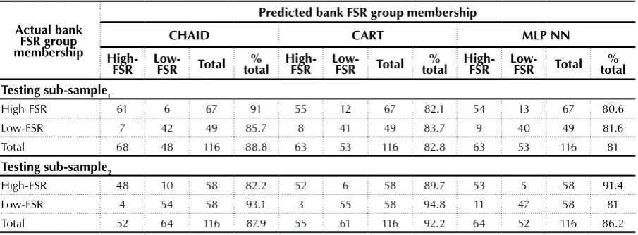
Classification results for bank FSR group mem-bership models using CHAID technique are summarized in Table 7. All the 17 financial and non-financial indicators for sub-sample1 and sub-sample2 are utilized. For the testing/hold-out sub-sample1, the overall average correct classification (ACC) rate is 88.8%. The predictive capabilities for high-FSR and low-FSR are 91% and 85.7%, respec-tively. Concerning testing sub-sample2, the overall ACC rate is 87.9% and the predictive capability of CHAID in foreseeing low-FSR rate of 93.1% is bet-ter than the high-FSR rate of 82.8%. Comparing different testing sub-samples, CHAID model us-ing sub-sample1 predicts 91% high-FSR which is better than the 85.7% low-FSR. By contrast, CHAID model using sub-sample2 predicts 93.1% low-FSR in comparison to only 82.2% high-FSR.
CART
CART is used to explore the anticipated differ-ences between the proposed models in relation to ACC rates using the same 17 financial and non-financial predictor indicators. Table 7 shows the classification for sub-sample1 and sub-sample2
for CART bank FSR group membership models. Concerning testing sub-sample1, the overall ACC rate is 82.8% with 82.1% and 83.7% for high-FSR and low-FSR, respectively. The overall ACC rate is lower than that associated rate under CHAID model (i.e. 88.8%) using the same sample. This significant decline in the ACC rate is a result of the lower predictive power of the CART model (i.e. 82.1% for high-FSR and 83.7% for low-FSR) compared to the CHAID model (i.e. 91% for high-FSR and 85.7% for low-high-FSR). For the testing sub-sample2, the ACC rate is 92.2% which is higher than that associated rate under CHAID model (i.e. 87.9%). This is a result of the better predictive accuracy rates of 89.7% and 94.8% for high-FSR and low-FSR, respectively using CART compared to 82.8% and 93.1% for high-FSR and low-FSR, re-spectively using CHAID.
Multilayer-Perceptron Neural
Networks
[image:13.595.73.526.100.267.2]MLP NNs are designed using the same 17 finan-cial and non-finanfinan-cial indicators under sub-sam-ple1 and sub-sample2. The overall ACC rate using testing sub-sample1 is 81% with 80.6% and 81.6% for high-FSR and low-FSR, respectively, as shown in Table 7. As for testing sub-sample2, the classifi-cation matrix shows that the overall ACC is 86.2%; in addition, MLP NN model predicts high-FSR (i.e., 91.4%) better than the low-FSR (i.e., 81%). The
Table 7. Classification results for the three machine learning modelling techniques
Actual bank FSR group membership
Predicted bank FSR group membership
CHAID CART MLP NN
High-FSR Low-FSR Total total % High-FSR Low-FSR Total total % High-FSR Low-FSR Total total %
Testing sub-sample1
High-FSR 61 6 67 91 55 12 67 82.1 54 13 67 80.6
Low-FSR 7 42 49 85.7 8 41 49 83.7 9 40 49 81.6
Total 68 48 116 88.8 63 53 116 82.8 63 53 116 81
Testing sub-sample2
High-FSR 48 10 58 82.2 52 6 58 89.7 53 5 58 91.4
Low-FSR 4 54 58 93.1 3 55 58 94.8 11 47 58 81
Total 52 64 116 87.9 55 61 116 92.2 64 52 116 86.2
increased overall ACC rate is a result of the higher predictive capability rate of 91.4% for high-FSR in testing sub-sample2, compared to a rate of 80.6% in sub-sample1.
3.2.2. Conventional techniques
Discriminant analysis
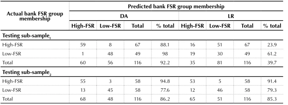
We run DA models using the same 17 financial and non-financial predictor indicators, and they are statistically significant at the 99% confidence level. As shown in Table 8, the overall ACC rate under testing sub-sample1 is 92.2% which is sur-prisingly the highest of all the techniques applied in this paper. The ACC rates for high-FSR and low-FSR are 88.1% and 98%, respectively. Clearly DA superiorly predicts low-FSR compared to all other techniques used in this paper. The classification results for testing sub-sample2 revealed that the overall ACC rate is 86.2% with 94.8% and 77.6% ACC rates for high-FSR and low-FSR, respectively,
as shown in Table 8.
Logistic regression
We also run LR models using the 17 financial and non-financial predictor indicators, and they are statistically significant at the 99% confidence level. As summarized in Table 8, the ACC rate associated with testing sub-sample1 is 39.7% which is the
low-est rate across all statistical techniques employed in our paper. In addition, this model has the low-est predictive power for high-FSR (i.e., 23.9%). Concerning testing sub-sample2, the overall ACC is 85.3% with 91.4% and 79.3% for high-FSR and low-FSR, respectively. Clearly sub-sample2 results show huge improvement compare to sub-sample1 results for this technique.
3.3. Comparison of different
models’ results
[image:14.595.70.532.99.268.2]Using testing sub-sample1 (i.e., predicting bank FSR group membership in 2007–2009), the highest ACC rate of 92.2% is associated with DA model; whilst using testing sub-sample2, the same ACC rate of 92.2% is associated with CART. All techniques predict low-FSR better than high-FSR group memberships using sub-sample1, except the CHAID model. However, for sub-sample2 (randomly predicting 33% of the overall sample), results are mixed. Both CHAID and CART predict low-FSR better than high-FSR, whilst the other three techniques namely MLP NN, DA and LR predict high-FSR bet-ter than low-FSR group memberships, as show in Tables 7 and 8. In order to compare different models predictive capabilities, estimates mis-classification cost (EMC) is used. The following equation (see for example, Abdou (2009b) is ap-plied in calculating the EMC:
Table 8. Classification results for the two conventional modelling techniques
Actual bank FSR group membership
Predicted bank FSR group membership
DA LR
High-FSR Low-FSR Total % total High-FSR Low-FSR Total % total
Testing sub-sample1
High-FSR 59 8 67 88.1 16 51 67 23.9
Low-FSR 1 48 49 98 19 30 49 61.2
Total 60 56 116 92.2 35 81 116 39.7
Testing sub-sample2
High-FSR 55 3 58 94.8 53 5 58 91.4
Low-FSR 13 45 58 77.6 12 46 58 79.3
Total 68 48 116 86.2 65 51 116 85.3
2 1,
L L H H
EMC E b E b
H H ⋅π + L ⋅ L π
= ⋅ ⋅ (10)
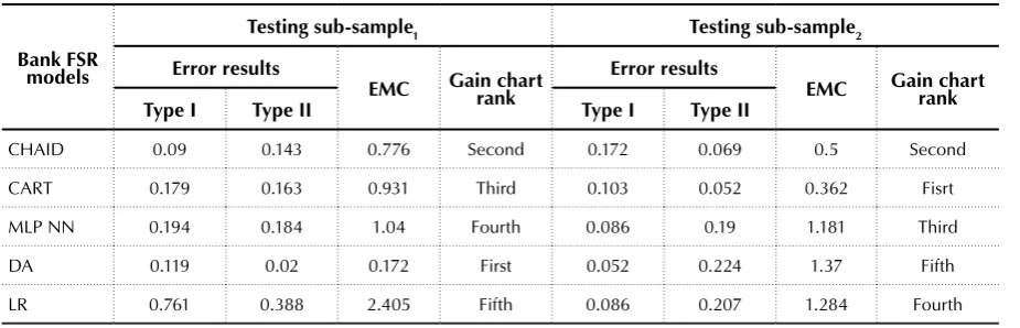
where, E (predicted low-FSR/actually high-FSR) and E (predicted high-FSR/actually low-FSR) refers to the corresponding EMC of Type I error and Type II errors; b (predicted low-FSR/actual-ly high-FSR) and b (predicted high-FSR/actually low-FSR) refers to the probabilities of Type I er-ror and Type II erer-rors; and π2 and π1 are prior probabilities of low-FSR and high-FSR, respec-tively. We use a ratio of 5:1 to present the EMC associated with Type II and Type I errors follow-ing, for example, Abdou et al. (2008) and Abdou (2009b). Table 9 summarizes the error rates namely Type I7and Type II8 errors and the EMC results
for all techniques under the samples namely sub-sample1 and sub-sample2.
For testing sub-sample1, CHAID’s Type I error rate is lower than Type II error rate achieving a EMC of 0.776. In contrast, for other statistical techniques namely CART, MLP NN, DA and LR, the lowest misclassification cost of 0.172 is surpris-ingly associated with DA. It is believed that this is due to the significantly low Type II error associ-ated with DA model, as shown in Table 9. Indeed, this result agrees with our previous findings using
7 High-FSR is misclassified as low-FSR. 8 Low-FSR is misclassified as high-FSR.
ACC rate where the DA model provides the high-est ACC rate of 92.2%, as shown in Tables 7 and 8. Concerning testing sub-sample2, the lowest EMC of 0.362 is associated with CART model. This re-sult also is confirmed using the ACC rate criterion where CART has the highest ACC rate of 92.2%, as discussed above, as shown in Table 7.
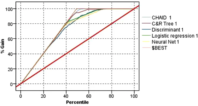
[image:15.595.70.533.112.261.2]For more details relating to testing sub-sample1 (predicting 2007–2009) and testing sub-sample2 (randomly predicting 33% of the overall sample), the reader is referred to Figure 3 and Figure 4; this illustrates our third criterion namely the gain chart using the machine leaning and conventional techniques applied in this paper, respectively. The gains chart is a valuable method of visualizing how good a predictive model is, as it plots the values in the Gain (%) column from the gains table. Gains refer to the increment number of hits divided by the overall number of hits multiplied by one hun-dred. If the models are not used, the ‘diagonal line’ plots the expected response in the testing sub-samples. The higher percentiles of gains, reflected in the curve line, represent how much the model can be improved with steeper curves representing higher gains. Visual gain charts analysis has in-deed confirmed our results for both sub-sample1 and sub-sample2 using other criteria, namely ACC rate and EMC.
Table 9. Error rates, estimated misclassification costs and gain chart ranking for all the five modelling techniques
Bank FSR models
Testing sub-sample1 Testing sub-sample2
Error results
EMC Gain chart rank Error results EMC Gain chart rank
Type I Type II Type I Type II
CHAID 0.09 0.143 0.776 Second 0.172 0.069 0.5 Second
CART 0.179 0.163 0.931 Third 0.103 0.052 0.362 Fisrt
MLP NN 0.194 0.184 1.04 Fourth 0.086 0.19 1.181 Third
DA 0.119 0.02 0.172 First 0.052 0.224 1.37 Fifth
LR 0.761 0.388 2.405 Fifth 0.086 0.207 1.284 Fourth
CHAID
CART
[image:16.595.67.521.85.442.2]DA
Figure 3. Gain charts for machine learning techniques using 2007–2009 testing sub-sample1 and 33% testing sub-sample2
MLP NN
LR
[image:16.595.70.521.495.722.2]CONCLUSION AND AREAS
FOR FUTURE RESEARCH
The assessment of the creditworthiness of banks and other financial institutions has become very chal-lenging due to structural changes in the global banking sector and the variability of creditworthiness within this sector. In addition, the financial crisis of 2007–2009 highlighted that banking systems are facing severe problems across different regions and that predicting ‘correct’ banks’ FSR group member-ship seems more important than ever. This paper presents how Middle Eastern banks can use machine learning techniques, namely CHAID, CART and MLP NN as well as conventional techniques, namely DA and LR to utilise financial and non-financial indicators to predict a bank’s FSR group membership.
Our results show that using testing/hold-out sub-sample1, DA model has the highest ACC rate of 92.2% and the lowest EMC of 0.172. This can be explained due to the minimal type II error rate. As for testing sub-sample2, CART has the highest ACC rate of 92.2% and lowest EMC of 0.362. Our gain chart results for both sub-samples do support the findings under the previous criteria, namely ACC rate and EMCs. In general, it can be concluded that DA as a conventional technique and CART as a machine learning technique are superior to all other techniques in predicting ‘correct’ bank’s FSR group membership in the Middle East region using data for the period 2007–2009 and for randomly selected sub-sample, respectively. Our future research can be extended in a number of ways. First, to investigate the prediction of high-FSR (and near high-FSR) versus low-FSR (and near low-FSR) during the Arab Spring commencing 2010. Second, to compare rated and non-rated banks to identify what non-rated banks need to achieve in order to secure higher rates. Third, apply other statistical model-ling techniques such as SVM and genetic algorithms. Finally, use cross-validation technique to reduce any possible inconsistencies in results.
REFERENCES
1. Abdallah, W. M. (2013). The im-pact of Financial and Non-Finan-cial mesures on Banks’ FinanNon-Finan-cial Strength Ratings: The Case of the Middle East (Ph.D. Thesis, Salford University, UK).
2. Abdou, H. A. (2009a). An Evaluation of Alternative Scoring Models in Private Banking. Journal of Risk Finance, 10(1), 38-53. https://doi. org/10.1108/15265940910924481
3. Abdou, H. A. (2009b). Genetic Programming for Credit Scoring: The Case of Egyptian Public Sector Banks. Expert Systems with Applications, 36(9), 11402-11417. https://doi.org/10.1016/j. eswa.2009.01.076
4. Abdou, H. A., Alam, S. T. & Mulkeen, J. (2014). Would credit scoring work for Islamic finance? A neural network approach.
International Journal of Islamic and Middle Eastern Finance and Management, 7(1), 112-125.
5. Abdou, H. A., Pointon, J., & El-Masry, A. (2008). Neural Nets versus Conventional Techniques in Credit Scoring in Egyptian Banks.
Expert Systems with Applications, 35(3), 1275-1292. https://doi. org/10.1016/j.eswa.2007.08.030
6. Abdou, H. A., Tsafack, M., Ntim, C., & Baker, R. (2016). Predicting creditworthness in retail banking with limited scoring data.
Knowledge-Based Systems, 103,
89-103. https://doi.org/10.1016/j. knosys.2016.03.023
7. Abdou, H., Pointon, J. (2009). Credit scoring and decision-making in Egyptian public sector banks. International Journal of Managerial Finance, 5(4), 391-406. 8. Akkoc, S. (2012). An Empirical
Comparison of Conventional Techniques, Neural Networks and the Three Stage Hybrid Adaptive Neuro Fuzzy Inference System (ANFIS) Model for Credit Scoring Analysis: The Case of Turkish Credit Card Data. European
Journal of Operational Research, 222(1), 168-178.
9. Altman, E. I. (1971). Corporate Bankruptcy in America. Heath Lexington Books.
10. Altman, E. I., & Sametz, A. W. (1977). Financial Crises: Institutions and Markets in a Fragile Environment. John Wiley & Sons Inc.
11. Bijak, K., & Thomas, L. C. (2012). Does Segmentation always Improve Model Performance in Credit Scoring? Expert Systems with Applications, 39(3), 2433-2442. https://doi.org/10.1016/j. eswa.2011.08.093
12. Brown, I., & Mues, C. (2012). An Experimental Comparison of Classification Algorithms For Imbalanced Credit Scoring Data Sets. Experts Systems with Applications, 39(3), 3446-3453. https://doi.org/10.1016/j. eswa.2011.09.033
Bank Failure via Multivariate Statistical Analysis of Financial Structures: The Turkish Case.
European Journal of Operational Research, 166(2), 528-546. 14. Chandra, D. K., Ravi, V., & Bose,
I. (2009). Failure Prediction of Dotcom Companies using Hybrid Intelligent Techniques. Expert Systems with Applications, 36(3), 4830-4837.
15. Chen, Y-S. (2012). Classifying credit ratings for Asian banks using integrating feature selection and the CPDA-based rough sets approach. Knowledge-Based Systems, 26, 259-270.
16. Chen, Y-S., & Cheng, C-H. (2013). Hybrid models based on rough set classifiers for setting credit rating decision rules in the global banking industry. Knowledge-Based Systems, 39, 224-239.
https://doi.org/10.1016/j.kno-sys.2012.11.004
17. Diomande, M. A., Heintz, J., & Pollin, R. (2009). Why U.S. Financial Markets Need a Public Credit Rating Agency. The Economist, 6(6), 1-4.
18. Falavigna, G. (2012). Financial Ratings with Scarce Information: A Neural Network Approach.
Expert Systems with Applications, 39(2), 1784-1792.
19. Hammer, P. L., Kogan, A., & Lejeune, M. A. (2012). A Logical analysis of Banks’ Financial Strength Ratings. Expert Systems with Applications, 39(9), 7808-7821. 20. Huang, Z., Chen, H., Hsu, C.-J.,
Chen, W.-H., & Wu, S. (2004). Credit Rating Analysis with Support vector machines and Neural Networks: A Market Comparative Study. Decision Support System, 37(4), 543-558. 21. Kao, L.-J., Chiu, C.-C., & Chiu, F.-Y. (2012). A Bayesian Latent Variable Model with Classification and Regression Tree Approach for Behavior and Credit Scoring.
Knowledge-Based Systems, 36,
245-252. https://doi.org/10.1016/j. knosys.2012.07.004
22. Kim, K.-J., & Ahn, H. (2012). A Corporate Credit Rating Model Using Multi-Class Support vector
machines with An Ordinal Pairwise Partitioning Approach.
Computers & Operations Research, 39(8), 1800-1811. https://doi. org/10.1016/j.cor.2011.06.023
23. Kolari, J., Glennon, D., Shin, H., & Caputo, M. (2002). Predicting Large US Commercial Bank Failures. Journal of Economics & Business, 54(4), 361-387.
24. Koyuncugil, A. S., & Ozgulbas, N. (2012). Financial Early Warning System Model and Data Mining Application for Risk Detection.
Expert Systems with Applications, 39(6), 6238-6253. https://doi. org/10.1016/j.eswa.2011.12.021
25. Kumar, P. R., & Ravi, V. (2007). Bankruptcy Prediction in Banks and Firms via Statistical and Intelligent Techniques- A Review.
European Journal of Operational Research, 180(1), 1-28.
26. Laere, E. V., Vantieghem, J., & Baesens, B. (2012). The Difference Between Moody’s and S&P Bank Ratings: Is Discretion in the Rating Process Causing a Split? (RMI Working Paper No. 12/05). 27. Lee, T.-S., Chiu, C.-C., Chou,
Y.-C., & Lu, C.-J. (2006). Mining the Customer Credit using Classification and Regression Tree and Multivariate Adaptive Regression Splines. Computational Statistics & Data Analysis, 50(4), 1113-1130.
28. Li, H., Sun, J., & Wu, J. (2010). Predicting Business Failure using Classification and Regression Tree: An Empirical Comparison with Popular Classical Statistical Methods and Top Classification Mining Methods. Expert Systems with Applications, 37(8), 5895-5904.
29. Loannidis, C., Pasiouras, F., & Zopounidis, C. (2010). Assessing Bank Soundness with Classification Techniques.
OMEGA, 38(5), 345-357.
https://doi.org/10.1016/j.ome-ga.2009.10.009
30. Oelerich, A., & Poddig, T. (2006). Evaluation of Rating Systems.
Expert Systems with Applications, 30(3), 437-447.
31. Pasiouras, F., Gaganis, C., & Doumpos, M. (2007). A
Multicriteria Discrimination Approach for the Credit Rating of Asian Banks. Annals of Finance, 3(3), 351-367. Retrieved from https:// link.springer.com/article/10.1007/ s10436-006-0052-0
32. Poon, W. P. H., & Firth, M. (2005). Are Unsolicited Credit Ratings Lower? International Evidence from Bank Ratings. Journal of Business Finance & Accounting, 32(9-10), 1741-1771.
33. Poon, W. P. H., Firth, M., & Fung, H.-G. (1999). A Multivariate Analysis of the Determinants of Moody’s Bank Financial Strength Ratings. Journal of International Financial Markets, Institutions and Money, 9(3), 267-283.
34. Poon, W. P. H., Lee, J., & Gup, B. E. (2009). Do Solicitations Matter in Bank Credit Ratings? Results from a Study of 72 Countries.
Journal of Money,Credit and Banking, 41(2-3), 285-314. http:// dx.doi.org/10.1111/j.1538-4616.2009.00206.x
35. Ravi, V., & Pramodh, C. (2008). Threshold Accepting Trained Principal Component Neural Network and Feature Subset Selection: Application to Bankruptcy Prediction in Banks.
Applied Soft Computing, 8(4), 1539-1548.
36. Ravi, V., Kurniawan, H., Thai, P. N. K., & Kumar, P. R. (2008). Soft Computing System for Bank Performance Prediction. Applied Soft Computing, 8(1), 305-315. 37. SPSSInc (2012). PASW Modeler 14
Algorithms Guide. Chicago: IBM SPSS Inc.
APPENDIX
Table A1. List of bank financial variables used in building the proposed bank FSR group membership models
Financial indicators Variables
Asset quality
The ratio of loan loss provision to net interest revenue (LLPNIR) The ratio of loan loss reserve to impaired loans (LLRIL) The ratio of impaired loans to gross loans (ILGL)
Capital adequacy
The total capital ratio (TCR) The ratio of equity to total assets (CS) The ratio of equity to net loans (ENL) The equity multiplier (EM)
Profitability
The net interest margin (NIM)
The ratio of non interest expense to total average assets (NIEAA) The recurring earning power ratio (REP)
The asset utilization ratio (AU)
The tax management efficiency ratio (TME)
Credit risk The ratio of loan loss provisions to total loans (LLPTL)
Liquidity The ratio of liquid assets to deposit and short term funding (LADSTF)*