A Multi-phase Mixture Theory for Debris Flows: Part I - Model Equations of Debris Flows

(1)

International Journal of Emerging Technology and Advanced Engineering

Website: www.ijetae.com (ISSN 2250-2459,ISO 9001:2008 Certified Journal, Volume 4, Issue 11, November 2014)

46

A Multi-phase Mixture Theory for Debris Flows: Part I - Model

Equations of Debris Flows

Huang Li-Jeng

1

, Hsiao Darn-Horng

2

Associate Professor, Department of Civil Engineering, National Kaohsiung University of Applied Science, 80778, Taiwan, Republic of China

Abstract—This paper presents the governing equations for analysis of debris flow based on the multi-phase mixture theory. The debris flow is considered to be a mixture of four constituents, i.e., stone, mud, water and air. Starting from the microscopic balance equations based on the theory of continuum mechanics and averaging theorems, the macroscopic balance equations are first built up to represent the conservation of mass, linear momentum, angular momentum, energy and entropy. After the constitutive relations are employed, the governing equations for debris flows are obtained. Mathematical model is completed when appropriate boundary conditions and initial conditions are prescribed. In special cases, the field equations will be degenerated to those corresponding to single phases. The proposed mathematical model can be employed for further theoretical analysis, computational simulation, and experimental verification of debris flow of different kinds.

Keywords—Balance Equations, Debris Flow, Governing Equations, Mathematical Models, Multi-phase Mixture Theory.

I. INTRODUCTION

Debris flow is a special type of hyper-concentrated flow, composed of mud, clay, sand, gravels, water, air and so forth, flowing down mainly due to its gravitational force. Natural disasters caused by debris flows often occur all over the world recently and there are many natural or manmade factors leading to these tremendous accidents [1, 2]. Development of prevention techniques is obviously based on the understanding and analysis of the mechanical behavior of debris flow [3, 4].

Some tremendous and famous disasters caused from debris flows from the past had been reported such as [5]: 1)(218 BC) Hannibal Barca, a Punic Carthaginian military

commander, led his army passed the mountains in the north of Italy to attack Rome but about 18 thousands of sodiers dead or hurt from rockfall [6, 7];

2)(1916) during World War I the Austrian and Italian armies attacked each other by bombarding the snowy crest of mountain and resulted in snowfall which led to 80,000 people dead.

3)(1966) a landslide occurred in Abergavenny of Wales results in destroy of elementary school and death of 116 children and 28 adults;

4)(1968) snowfall occurred in Dakfose, Switzerland led to death of 53 people. Then an institute was established and debris dams were built to circumvent the disaster; 5)(1978) in Lisa, Norway, landslide occurred due to

liquefaction led to disappear of half of a village; 6)(1985) the liquefaction failure of two tailing dams in the

Stava Creek Valley, North-Eastern Italy caused an extremely debris flow which wiped out and/orburied two villages and claimed 270 lives.

7)(1991) in Fukuoka, Japan, a volcano exploded with ash up to 150 mile, the pyroclastic flow attacked village located at downstream and resulted in death of 43 people;

8)(1995) in Iceland, an icefall destroyed 50 houses and resulted in death of 20 people;

9)(2007) storm induced landslide occurred in Jawa, Indonesia killed at least 77 people; while debris flow occurred in Flores island killed at least 40 people. 10) (2008) landslide occurred in Lao-Cai Province,

Vietnam and at least 62 people killed.

11) (2009) mudslide occurred in Patung, Indonesia killed at least 644 people.

12) (2010) mudslide appeared in the Zhu-gqu of Gan-Su Province of China killed 1481 people and made 284 disappeared together with a village with 300 houses embedded under the mud. A debris lake was formed and induced secondary disaster later.

13) (2011) continuous storm and rainfall induced debris flow in Chuncheon, Seoul, Korea and killed13 people. 14) (2014) mudslide occurred in Washington D. C. killed

24 people and more than 90 people disappeared.. 15) (2014) landslide occurred in the Fu-Chan City of

Quae-Zou Province of China led to 7 people dead, 20 disappeared and 22 hurt.

16) (2014) landslide occurred in the village of Malin in Maharashtra, India killed at least 160 people.

(2)

International Journal of Emerging Technology and Advanced Engineering

47

18) (2014) mudslide occurred in Sindhupalchowk of Nepal

resulted in 9 people dead and hundreds of people disappeared.

19) (2014) Oso mudslide occurred in Washington State, U.S.A. causes 43 deaths and 49 homes destroyed.

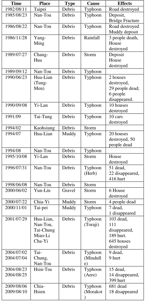
Table I summarizes some disasters caused by debris flows in Taiwan [5, 8]. It should be noticed that in Japan a 20-years statistical data from 1967 to 1987 reported that among total 4597 dead people caused from natural disaster, 1257 (27.3%) dead people were due to debris flows.

Debris flows are inherently non-Newtonian flows from the viewpoints of view of fluid mechanics, in which the rheological behavior is highly nonlinear and complicated. On the other hand, from the viewpoints of solid mechanics, debris flows are porous media filled with water, air and other slurries.

There have been a lot of flow models for analysis of mechanical characteristics of debris flow. Among these research works, the following models are useful and significant: the dilatant fluid model initiated by Bagnold (1954) [9] and extended by Takahashi (1977, 1978) [10, 11]; the Bingham fluid model, pseudo- or generalized visco-plastic fluid model such as those proposed by Chen (1986) [12], O’Brien and Julien (1988) [13], Chen et al. (1991) [14], Julien and Lan (1991) [15], etc.; Prandtl mixing-length model employed by Matsumura and Mizuyama (1990) [16]; modified turbulent flow model proposed by Yu and Chen(1990) [17]; a mixed-layer model proposed by Su et al (1993) [18] in which an inertia sub-region and a viscous sub-sub-region exist. It has been found by experimental study that the Bingham fluid model is appropriate for mud flow while dilatant fluid model works well for stony flow in which dispersive stresses together with the viscous shear stresses play the same role in the rhelogical behavior of the debris flow.

Thus it is naturally to develop a rheological model based on the theory of multi-phase mixture, in which the debris flow is considered to be a mixture of four constituents, i.e., stone, mud, water and air. In the analysis of geophysical and geotechnical problems, theories of multi-phase mixture have been employed for a long time (Hassanizadeh et al. 1979, 1980; Lewis,and Schrefler, 1998; Zienkiewicz et al., 1999; Li, Xi-Kui and Ziekiewicz, 1992) [19-24]. There are two basic points of view on the multi-phase mixture, i.e., the microscopic and the macroscopic, respectively. On the other hand, concept of effective stress has been employed by Terzaghi (1936) [25] and extended by Biot (1941, 1956) [26, 27].

TABLEI

SOME DISASTERS CAUSED BY DEBRIS FLOWS IN TAIWAN

Time Place Type Cause Effects

1982/08/11 Taipei Debris Typhoon Road destroyed 1985/08/23 Nan-Tou Debris Typhoon Deposit,

Bridge Fracture 1986/08/22 Nan-Tou Debris Typhoon Road destroyed Muddy deposit 1986/11/28

Yang-Ming

Debris Rainfall 3 people death, House destroyed 1989/07/27

Chang-Hua

Debris Storm Deposit House destroyed 1989/09/12 Nan-Tou Debris Typhoon

1990/06/23 Hua-Lian (Tung-Men)

Debris Typhoon 2 houses destroyed, 29 people dead; 6 people disappeared. 1990/09/08 Yi-Lan Debris Typhoon 10 houses

destroyed 1991/09 Tai-Tung Debris Typhoon 10 cars

destroyed 1994/02 Kaohsiung Debris Storm

1994/07 Hua-Lian Muddy Typhoon 20 houses destroyed, 50 people dead 1994/08 Nan-Tou Debris Typhoon

1995/10/08 Yi-Lan Debris Storm House destroyed 1996/07/31 Nan-Tou Debris Typhoon

(Herb)

51 dead, 22 disappeared, 416 hurt 1998/06/08 Nan-Tou Debris Storm

2000/06/02 Yun-Lin Gravel Storm 6 House destroyed 2000/07/22 Chia-Yi Muddy Storm 4 people dead 2000/11/01 Tai-pei Muddy Typhoon 7 dead,

1 disappeared 2001/07/29 Hua-Lian,

Nan-Tou, Tai-Chung Miao-Li Cha-Yi

Debris Typhoon (Toraji)

103 dead, 111 disappeared, 189 hurt. 645 houses destroyed 2004/07/02

2004/07/04 Tai-Chung, Nan-Tou

Debris Typhoon (Mindull e)

9 dead, 9 hurt 2004/08/23

2004/08/25

Hsin-Tsu Debris Typhoon (Aere)

15 dead, 14 disappeared, 399 hurt 2009/08/06

2009/08/10 Chia-Hsien

Debris Typhoon (Morakot )

[image:2.612.323.564.158.661.2]

(3)

International Journal of Emerging Technology and Advanced Engineering

48

Once the constitutive relationship is built up we can theoretically evaluate the kinematic characteristics of debris flow along a slope such as velocity profile, mean velocity, plug velocity, momentum correction factor and energy correction factor, etc. Special cases for degenerating condition can also be obtained in a simple way.

II. BASIC PROPERTIES OF DEBRIS FLOWS

A. Classification of Debris Flows

According to the particle sizes of major contents, debris flow can be classified into three categories:

1)Mud flow: particles of the size less than 0.1 mm are more than 50%;

2)Mud-Rock flow (mixed flow): particles of the size less than 0.1 mm are between 10% and 50%;

3)Granular flow (stony flow)(rock flow): particles of the size less than 0.1 mm are less than 10%.

The three types of debris flow are quite different in nature. The mud flow may cause less collision force but it may result in tremendous loss of life due to its silence of flow motion without precaution. On the other hand, granular flow usually accompanies with giant sound and huge stones that looks like a group of rock motions

(Coussot , 1997; Cheng et al. 1997) [28, 29].

Furthermore, Takahashi (2000) [30] proposed a ternary diagram to describe four kinds of debris flow based on the values of Reynolds number, Re, Bagnold number, Ba, and relative depth of flow, h/d. The typical stony, muddy and viscous types of debris flows occur in the domain s near the apexes; the rest of area is the domain of hybrid-debris flows.

B. General Features of Debris Flows

The general features of debris flows can be summarized as follows:

1)the size distribution of debris flow ranges widely from 0.01 mm to some meters;

2)mass per unit volume (specific density) of debris flow ranges from 1400 kg/m3 to 2300 kg/m3;

3)most of debris flows occur at slope angle between 15o and 30o;

4)the thickness of deposit ranges from some centimeters to some meters and the average is 2 m;

5)re-occurrence of debris flow in a region usually exists; 6) three regions usually exist in a debris flow:

(a) Generation Region (Source Area). (b) Transportation Region (Flow Track). (c) Deposition Region (Stoppage Area).

C. Moving Features of Debris Flows

Debris flow contains parts of features of fluids and its special moving features can be explained as follows:

1)a type of discontinuous intermittence fluid flow exists; as the front part blocked, stopped and dried, the new coming flow push the front part moving again due to inertia effect;

2)the front of debris flow usually forms wave motion accompanying with coarse particles while minor and lighter particles distributed in the aft part;

3)the cross-section in the front part is in the form of bell (convex) shape while in the aft part bowel shape (concave);

4)in general the surface velocity is greater than that of bottom velocity and average velocity; average velocity of mud flow ranges in 2-20 m/sec; while granular flow ranges in 3-10 m/sec;

5)flow motion is nearly straightforward containing moving, rolling, sliding and jumping.

D. Sliding Features of Debris Flows

Sliding features of debris flow originates from its solid and particle contents. During this process sectional waves, collision, inter-shear and dehydration may occur.

E. Deposition Features of Debris Flows

Deposition is a specific feature of debris flow which is quite different from water flows. These deposition features are:

1)debris fan forms at the end area of debris flow, due to increasing width and decreasing depth, and its width is about 2~3 multiples of the width of valley;

2)flat-type lobe (tongue-shaped) or swollen-type lobe usually form;

3)debris flow with coarse particles can form larger arrival distance.

F. Mechanical Behaviors of Debris Flows

In general debris flow contains solids, fluids, gases and depicts complicated mechanical behaviours. These mechanical behaviours are summarized as follows:

1)it is a kind of multi-phase flow: solid-phase contents (Stones, sands, soils and silts, etc.) as well as fluid-phase contents (water, air, and oil, etc.)

(4)

International Journal of Emerging Technology and Advanced Engineering

49

3)it becomes creeping flow if flow is in slow motion;

while when the inertia effects become important wave motion occurs;

4)constitution relationships are complicated and change with time and cannot be identified by fixed unified formula. Special formula is valid for typical flows. It is near the elasto-plastic and plastic materials.

III. BALANCE EQUATIONS FOR MULTI-PHASE SYSTEM

G. Microscopic balance equations

From the classical balance equations of continuum mechanics, the generic conserved variable  within the  phase can be written as

G b r

t   



         

i ) ( ) (

 (1)

Where  is the density, r is the local value of the velocity field of the  phase, i is the flux vector associated with  , b,Gare the external supply and net

production of  , respectively.

At the interface between two adjacent phases and ,

the jump conditions hold











 

 

(wr)i n  (wr)i n (2)

Where w is the velocity of the interface, n denotes the unit normal vector pointing out the  phase into the

phase.

The generic conserved variables for mass, momentum, energy and entropy are 1,r,E0.5rr,, respectively.

H. Averaging principle

The volume fraction of the



phase is defined as

dV t r dV H dV dV dV t

x, ) 1 ( , )

(     

 

 (3)

Where H is the phase distribution function defined as

  

dV dV t

r H

  

r for 0

r for 1 { ) ,

( _

 

(4)

And x,r represents the position of a representative elementary volume in a global system and the position of a microscopic volume element, respectively.

The area fraction of the phase is defined as

dA t r dA H dA dA dA t

x, ) 1 ( , )

(     

 

 (5)

Here the suggested identity is employed:

) , ( ) ,

(x t  x t 

  (6)

In order to deduce the macroscopic balance equations, the following averaged quantities are defined:

(i)volume average operator and intrinsic volume average operator are defined by:

t)dV H

t dV f dV t

f _(x, ) 1  (r, ) (r, (7)

and

t)dV H

t dV f dV t

f (x, ) 1 (r, ) (r, 



   (8)

(ii)The mass average operator is defined as

 

t)dV H

t dV t f

t)dV H

t dV

t)dV H

t dV t f t

f

r, ( ) , r ( ) r, ( 1

r, ( ) , r (

r, ( ) , r ( ) r, ( )

, x (

 



 

  

(9)

(iii)The area average operator is defined as

t)dV H

t dA dA t

f _(x, ) 1  f(r, )n (r, (10)

I. Macroscopic balance equations

Applying the averaging operators and averaging theorems depicted by Hassanizadeh and Gray (1979), we can obtain the following macroscopic balance equations for multiphase system without phase exchange:

 

_   _

 

_

 

 

    

  

G I

b t

  

   

  



) (

i ) ] v [ ( ) (

(11)

subjected to

V I

N

  

 ( ) 0 x

(5)

International Journal of Emerging Technology and Advanced Engineering

50

Hence the equations of balance for a multi-phase system from the classical equations of continuum mechanics for each phase are:

Conservation of mass

 

v 0 



  _ _

  

 Dt

D

(13a)

Conservation of linear momentum:

 

_{ }

0

T g

t v



 

 

   _ _  _ 

  

 



Dt D

(13b)

Conservation of angular momentum:

) (

T t

t symmetric (13c)

Conservation of energy:

 

0

q v

: t

 



    

     

 

    

Q h

Dt E

D  

(13d)

Entropy balance:

 

_

 

 

    

 

  

 

  

 q h

Dt S D

) (



(13e)

subjected to

0 T 1

 



 

 

N

(14a)

 

v ) 0 T

( 1

   



   

  Q

N

(14b)

Where  _ is the volume average of density of the 

phase (i.e., the mass of  phase per total volume of the multiphase system),

 

v_ is the intrinsic mass average

velocity of the  phase, t is the stress tensor of the  phase,

 

g_ is the -phase external supply of momentum

related to gravitational effect, T is the exchange of momentum between the -phase and all other phases due

to mechanical interaction, Eis the -phase macroscopic

internal energy density function, q is the -phase heat flux, h is the -phase external supply of energy, Q is the exchange of internal energy between -phase and all

other phases due to mechanical interactions,

 

S_ is the

-phase internal entropy density function,  is the  -phase absolute temperature function,

 

_ is the  -phase

net production of entropy, the material differential operator

) ( /

) ( / )

(    

 _f _Dt _f _t _grad _f _v

D     , i.e. he time derivative is taken moving with the phase.

For simplicity these averaging symbols will be omitted in the remainder of the present work.

IV. MODEL EQUATIONS FOR DEBRIS FLOWS

A. Basic Assumptions

In the formulation of the governing equations of debris flow the following assumptions are employed:

(1)The constituents are assumed to be immiscible and chemically non-reacting;

(2)All fluid phases (water and air) are assumed to be in contact with the solid phases;

(3)Isothermal conditions in each phase is hold;

(4)The real multiphase system that occupies the porous medium domain is replaced by a model in which each phase is assumed to fill up the entire domain;

(5)Heat conduction and vapour diffusion, heat convection and transfer due to fluid phase change;

(6)There exist no surface continuity at the macroscopic scale;

(6)

International Journal of Emerging Technology and Advanced Engineering

51

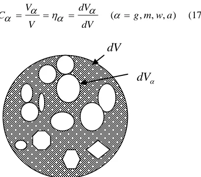
B. Macroscopic Balance Equations for Debris Flows

The debris flow is considered to be a multi-phase mixture composed of four constituents, i.e., gravel (stone), mud (sand), water and air (Figure 1). Thus the density of the mixture can be expressed as

   

        

  

 

 

4

1

a a w w m m g g

(15)

Where _g,_m,_w,_a denotes the density of

gravel(stone), mud(sand), water and air, respectively; and

a w m

g   

 , , , denotes volume fraction of gravel(stone), mud(sand), water and air, respectively. It is obviously seen that

1 4

1    i 

 (16)

For a mixture of immiscible solids and fluids it is reasonable to use the volume fraction in the whole volume to replace the volume fraction of a representative element volume, i.e.,

) , , , ( g m w a dV

dV V

V

[image:6.612.357.544.117.333.2]

C_   _     (17)

Figure 1 Typical representative element of multi-phase mixture of debris flow (1,2,3,4 denotes g,m,w,adescribing stone, mud,

water and air).

Figure 2 Typical phase diagram of debris flow.

Substituting (15) into (13) we have the following macroscopic balance equations in indicial form:

0 , )

(



__ 

    

k k v Dt

D

(18a)

0

.   

  __  _  

    

l T l g k

kl t Dt

l v D

(18b)

 

lk t kl

t  (18c)

0 , ,

 



 

         

        

Q h

k k q k l v kl t Dt

E D

(18d)

      

     

  qk _k  h  

Dt S D

, ) (

(18e)

subjected to

0 4

1

 



    

 Tl (19a) 

dV

V

Vw

Vg Va Air

Water

Mud (Sand)

Gravel (Stone)

[image:6.612.86.284.427.602.2]

(7)

International Journal of Emerging Technology and Advanced Engineering

52

0 ) ( 4 1         

  Tl vl Q (19b)

When the temperature in each phase is the same (isothermal condition), i.e.,

   

_g  _m _w _a (20)

As a result, energy equations for each phase need not be considered. Rather a total energy equation obtained as the sum of each phase energy equations will be

0 , ) ( , 4 1 , [        h k k v E k k q k l v kl t Dt DE             (21) where    4 1   

E E (22)

and    4 1    

h h (23)

C. Constitutive Equations for Debris Flows

The balance equations given in equations (18), (19) and (21) constitute equations in 48 unknowns, namely:

) 3 , 2 , 1 , ; 4 . 3 , 2 , 1 ( , , , , , 

 k l

S E kl t k v         (24)

However, some dependent variables can be related to others based on the so-called constitutive relations of each phase of the constituents.

(i)If the solid phase is assumed to be isotropic elastic, then

) , ( 2 m g S S kl e S kl S mn e S kl S p S S kl t           (25a) Where kl

 is the Kronecker delta, e_klS is the tensor of

the rate of deformation of solid phases, S,S are Lame constants of solid phases.

(ii)For Newtonian fluid (such as water and air phases):

) , ( 2 a w f f kl e f kl f mm e f kl f p f kl t          (25b)

Where e_klf is the tensor of the rate of deformation of

fluid phases, f ,f are Lame constants of fluid phases.

(iii)If the mud is assumed to be a Bingham fluid:

m l k v m m Y m kl t ,   

 (25c)

in which m _m

Y 

 , denote the yield stress and viscosity of the non-Newtonian fluid, respectively.

(iv)If the stony phase is assumed to be dilatant fluid:

2 ) , ( 2 2 ) sin

(a _gd_s u_kg_l

g kl

t     (25d)

Where a being a constant,  the kinetic friction of sediment, _g the density of sediment, d_sthe diameter of

particle of sediment, the characteristic length related to the concentration. This is a generalized dilatant fluid model based on the work of Bagnold (1954) [9] and Takahashi (1977, 1978) [10, 11] and is a nonlinear constitutive model.

(v)If the inertia and macroscopic viscous effects are neglected, the fluid-phase momentum equation can be simplified to be

) ,

(pf_k _fg_k f

lk K f l

v   (25e)

in which K_lkf is the permeability of the sediment, pf is the pressure of the fluid. This is the Darcy’s law valid as a first approximation for the slow flow of a macroscopically inviscid fluid through a non-uniform anisotropic elastic porous solid composed of incompressible grains.

D. Initial Conditions

In unsteady debris flow problems the initial conditions are needed, the form is as follows:

(8)

International Journal of Emerging Technology and Advanced Engineering

53

E. Boundary Conditions

There are different boundary conditions needed be taken into consideration:

(i)Dynamic boundary conditions:

The velocity vector of the debris flow at the wall must be equal to the velocity of the wall, i.e.,

U W k u t W x k

u( , ) at  (27)

(ii)Traction boundary conditions:

In the situation of traction boundary conditions such as at free surface, the boundary conditions read

T l t t W x k n kl

t ( , ) at  (28)

TABLEII

NUMBER OF UNKNOWNS AND EQUATIONS FOR MATHEMATICAL MODELING OF DEBRIS FLOW BASED ON MULTI-PHASE MIXTURE

THEORY

Eq. Eq. No.

No. of Eq.

Unknown Symbol No. of Unknown Continuity (18a) 4 Density _ 4

Linear Momentum

(18b) 12 Velocity 

k

v 12

Angular Momentum

(18c) 24 Stress _

kl

t 24

Energy (18d) 4 Internal Energy Density



E 4

Entropy (18e) 4 Internal Entropy Density



S 4

Summation 48 48

Table II summarize the number of equations and unknowns for a general problem of debris flow. These 48 governing equations accompany the boundary conditions, (27), and/or the initial conditions, (28), comprise a well-defined boundary value problem (BVP) and/or initial-boundary value problem (IBVP).

V. TYPICAL EXAMPLE OF MODEL EQUATIONS OF DEBRIS

FLOW

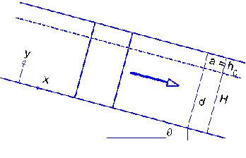
To explain how to use the model equations of debris flow based on multiple-phase mixture theory we consider a special simplified case of two-dimensional steady incompressible debris flow in x-y plane moving along an

[image:8.612.361.535.165.277.2]

infinite slope with angle  relative to the horizon (Figure 3).

Figure 3 Illustration of debris flow along a slope

As is often the case we assume that there are only three phases exist, i.e. the debris flow composed of gravel (stone), mud (sand) and water. The velocity components of each

phase is denoted by v (u,v) , .

3 , 2 , 1 

 Considering there is no momentum exchange between phases as well as no external heat input and the temperature is kept constant.

The governing equations thus can be expressed as follows:

(1) Conservation of mass of each phase:

Since it is assumed to be steady, (f)/t0, and

thus D(f)/Dtgrad(fv) . Furthermore,

incompressible assumption leads to __v_k_,_k 0. The conservation of mass, Eq. (18a) can be simplified to

) 2 , 1 , )( 3 , 2 , 1 ( , 0

,j   k j k

v 

  

 (18a’)

Which for ease phase becomes

(a) gravel (stone) phase:

0 )

( 

    

y g v x

g u g g

 (29a)

(b) mud (sand) phase:

0 )

( 

    

y m v x

m u m m

(9)

International Journal of Emerging Technology and Advanced Engineering

54

(c) water phase:

0 ) (       y w v x w u w w

 (29c)

(2) Conservation of linear momentum of each phase:

0 .     __        l g k kl t Dt l v D (18b’)

(a) gravel (stone) phase:

    

 ) ( ) sin

( : g g g y g XY Dt g u g D g g direction x   

 (30a)

 

  

 ) ( ) cos

( : g g g y g YY y p Dt g v g D g g direction y       

 (30b)

(b) mud (sand) phase:

 

  

 ) ( ) sin

( : g m m y m XY Dt m u m D m m direction x   

 (31a)

 

  

 ) ( ) cos

( : g m m y m YY y p Dt m v m D m m direction y       

 (31b)

(c) water phase:

 

  

 ) ( ) sin

( : g w w y w XY Dt w u w D w w direction x   

 (31a)

 

  

 ) ( ) cos

( : g w w y w YY y p Dt w v w D w w direction y       

 (31b)

Furthermore, for the convenience of analysis, we assume that the velocity components of each phase are the same in

macroscopic point of view; i.e., ug um uw u

andwg wm ww w,

(1) Conservation of mass of mixture of debris flow: Summation of Eq. (29a), (29b) and (29c) leads to

0 ) )( (         y v x u w w m m g

g    

 (32)

(2) Conservation of linear momentum mixture of debris flow:

Similarly, summation of Eq. (30a), (31a), (32a) leads to

              sin ) ( 0 ) ( : g w w m m g g y XY Dt Du w w m m g g direction x         

 (33a)

and summation of Eq. (30b), (31b), (32b) leads to

             cos ) ( 0 ) ( : g w w m m g g y p Dt Dv w w m m g g direction y        

 (33b)

The shearing stresses _XZ can be expressed as a function of velocity gradients from various constitutive relationships of debris flow models, Eq. (25).

Eqs. (32), (33a) and (33b) constitute the governing equations for two-dimensional steady incompressible debris flow made of three phases, gravel (stone), mud (sand) and water driving from the multi-phase mixture theory.

VI. CONCLUDING REMARKS

(10)

International Journal of Emerging Technology and Advanced Engineering

55

The proposed mathematical model can be employed for further theoretical analysis, computational simulation, and experimental verification.

Acknowledgement

This work is supported by the National Science Council of ROC through grant NSC 89-2211-E151-010.

REFERENCES

[1] Alexander, D. 1993. Natural Disasters, Univ. College London. [2] Chapman, D. 1994. Natural Hazard, Oxford Univ.

[3] Takahashi, T. 1991. Debris Flow, Balkema, Rotterdam.

[4] Jan, C. D. 2000. Introduction to Debris Flows, Science and Technology Books Company, Taiwan, R. O. C. (in Chinese). [5] Huang, L. J. 2001. Introduction to Theory and Practice of

Debris-Flow Hazards Mitigation, Chuan-Hwa Publishing Ltd., Taiwan, R.O.C. (in Chinese).

[6] Livy History of Rome, Book 21, sections 32-36.

[7] Mahaney, W. C. et al. 2009. The Traversette rockfall: geomorphological reconstruction and importance in interpreting classical history. Archaeometry, 52(1), 156-172.

[8] Lin, H. M. 2004. The Spatiotemporal Characteristics on the Natural Disasters in the Past Thirty Years in Taiwan. Geogra. Res. 41, 99-128.

[9] Bagnold, R. A. 1954. Experiments on a Gravity-Free Dispersion of Large Solid Spheres in a Newtonian Fluid Under Shear. Proc. of Royal Soc. of London, Ser. A. 225, 49-63.

[10] Takahashi, T. 1977. A Mechanism of Occurrence of Mud-Debris Flow and Their Characteristics in Motion. Annuals, Disaster Prevention Res. Inst., Tokyo University, 20B(2), 405-435 (in Japanese).

[11] Takahashi, T. 1978. Mechanical Characteristics of Debris Flow. J. of Hydrau. Div., ASCE, 104(HY8), 1153-1169.

[12] Chen, C. L. 1986. Generalized Visco-Plastic Modeling of Debris Flow,” J. of Hydrau. Engng., 114(3), 237-258.

[13] O’Brien, J. S. and Julien, P. Y. 1988 Laboratory Analysis of Mud flow Properties. J. of Hydrau. Engng., 114(8), 877-887.

[14] Chen, C.L., Lin, C. H. and Jan, C. D. 1991. Rheological Model for Ring-Shear Type Debris Flows. Proc. of the 5th Fed. Inter. Sedi. Conf. (5) 1-8.

[15] Julien, P. Y. and Lan, Y. 1991. Rheology of Hyperconcentrations. J. of Hydrau. Engng. 117, 346-353.

[16] Matsumura, K. and Mizuyama, T. 1990. Experimental Study on Mechanism of Debris Flow Using Light Materials. Shin-Sabo, 43(1), 16-22.

[17] Yu, F. C. and Chen, C. G. 1990. Basic Study on the Debris Flow: (II) Preliminary Study on the Flow Velocity of Debris Flow. J. Soil & Water Cons. 21-22(2), 115-142. (in Chinese).

[18] Su, C. G., Lien, H. P. and Chiang, Y. C. 1993. Study on the Velocity Distribution of Debris Flow. J. Chi. Soil & Water Cons. 24(1), 75-82. (In Chinese)

[19] Hassanizadeh, M. and Gray, W. G. 1979. General Conservation Equations for Multiphase Systems: 1. Averaging Procedure,” Adv. in Water Res.. 2, 131-144.

[20] Hassanizadeh, M. and Gray, W. G. 1979. General Conservation Equations for Multiphase Systems: 2. Mass, Momenta, Energy, and Entropy Equations. Adv. in Water Res. 2, 191-203.

[21] Hassanizadeh, M. and Gray, W. G. 1980. General Conservation Equations for Multiphase Systems: 3. Constitutive Theory for Porous Media Flow,” Adv. in Water Res. 3, 25-40.

[22] Lewis, R. W. and Schrefler, B. A. 1998. The Finite Element Method in the Static and Dynamic Deformation and Consolidation of Porous Media, Chapter 2, John-Wiley & Sons, Ltd.

[23] Zienkiewicz, O. C., Chan, A. H. C., Chan, Pastor, M., Schrefler, B. A., and Shiomi, T. 1999. Computational Geomechanics with Special Reference to Earthquake Engineering, Chapter 2, John Wiley & Sons Ltd.

[24] Li, Xi-Kui and Ziekiewicz, O. C. 1992. Multiphase flow in deforming porous media and finite element solutions. Computers & Structures, 45(2), 211-227.

[25] Terzaghi K. von, 1936. The shearing resistance of saturated soils, Proc. 1st ICSMFE, 1, 54-56..

[26] Biot, M. A. 1941. General theory of three-dimensional consolidation,” J. of Appl. Phy. 12, 155-164.

[27] Biot, M. A. 1956. General solution of the equation of elasticity and consolidation for a porous material. J. of Appl. Mech., 23, 91-96. [28] Coussot, P. 1997. Mudflow Rheology and Dynamics. Balkema,

Rotterdam.

[29] Cheng, J. D., Wu, H. L. and Chen, L. J. 1997. A Comprehensive Debris Flow Hazard Mitigation Program in Taiwan. Debris-Flow Hazards Mitigation: Mechanics, Prediction, and Assessment, ASCE, N. Y., 93-102.