Parallel hybrid viscosity method for fixed point problems, variational inequality problems and split generalized equilibrium problems

(1)

R E S E A R C H

Open Access

Parallel hybrid viscosity method for ﬁxed

point problems, variational inequality

problems and split generalized equilibrium

problems

Qingqing Cheng

1*

*_{Correspondence:}

[email protected]

1_{Department of Science, Tianjin}

University of Commerce, Tianjin, P.R. China

Abstract

In this paper, we first propose a new parallel hybrid viscosity iterative method for finding a common element of three solution sets: (i) finite split generalized equilibrium problems; (ii) finite variational inequality problems; and (iii) fixed point problem of a finite collection of demicontractive operators. And we prove that the sequence generated by the iterative scheme strongly converges to a common solution of the above-mentioned problems. Also, we present numerical examples to demonstrate the effectiveness of our algorithm. Our results presented in this paper improve and extend many recent results in the literature.

Keywords: Split generalized equilibrium problems; Variational inequality problems; Fixed point problems; Parallel hybrid viscosity method; Lipschitzian mappings

1 Introduction

LetH1andH2be two inﬁnite dimensional real Hilbert space with inner product and norm

denoted by·,·and · , respectively. LetCandQbe a nonempty closed convex subset

ofH1 andH2, respectively. LetT:C→Cbe a mapping. The set of ﬁxed points ofT is

denoted byF(T), that is,F(T) ={x∈C:Tx=x}.

In what follows, we recall some deﬁnitions of classes of operators often used in ﬁxed point theory.

Deﬁnition 1.1 LetT:C→Cbe a mapping. Then

(i) T isρ-Lipschitzianwithρ> 0if

Tx–Ty ≤ρx–y, ∀x,y∈C;

Ifρ∈(0, 1), thenTisρ-contractiveand ifρ= 1, thenTisnonexpansive. (ii) T isﬁrmly nonexpansiveif

Tx–Ty2≤ x–y2–(I–T)x– (I–T)y2, ∀x,y∈C;

(2)

(iii) Tisκ-strictly pseudo-contractivewithκ∈[0, 1)if

Tx–Ty2≤ x–y2+κ(I–T)x– (I–T)y2, ∀x,y∈C.

Deﬁnition 1.2 LetT:C→Cbe a mapping withF(T)=∅. Then

(i) Tisdirectedif

Tx–z2≤ x–z2–x–Tx2, ∀z∈F(T),x∈C;

(ii) Tisquasi-nonexpansiveif

Tx–z ≤ x–z, ∀z∈F(T),x∈C;

(iii) Tisβ-demicontractivewithβ< 1if

Tx–z2≤ x–z2+βx–Tx2, ∀z∈F(T),x∈C.

Note that the class of demicontractive operators contains important classes of operators:

directed operator (ﬁrmly nonexpansive operator with nonempty ﬁxed points set) forβ=

–1, quasi-nonexpansive operator (nonexpansive operator with nonempty ﬁxed points set)

forβ = 0, and strictly pseudo-contractive operator with nonempty ﬁxed points set for

β∈(0, 1); the class of quasi-nonexpansive operators also contains nonspreading mappings

with nonempty ﬁxed point set andN-generalized hybrid mappings with nonempty ﬁxed

point set.

It is well known that every nonexpansive operatorT:H1→H1satisﬁes the following

inequality;

(I–T)x– (I–T)y,Ty–Tx≤1

2(I–T)y– (I–T)x

2

,

for allx,y∈H1. Therefore, for allx∈H1,y∈F(T),

(I–T)x,y–Tx≤1

2(T–I)x

2

. (1.1)

We also know thatF(T) of nonexpansive mappingTis closed and convex.

The ﬁxed point problem (FPP) for the mappingTis to ﬁndx∈Csuch that

Tx=x.

Many iterative algorithms has been introduced for finding fixed points of nonexpansive mappings, quasi-nonexpansive mappings, firmly nonexpansive mappings,

demicontrac-tive mappings (see [1–6]), including the since recently popular viscosity iterative

algo-rithms, which formally consist of the sequence{xn}given by the iteration

xn+1=αnf(xn) + (1 –αn)Txn, ∀n≥0, (1.2)

wheref is a contraction,{αn} ⊂(0, 1) is a slowly vanishing sequence, i.e.,limn→∞αn= 0

(3)

whenf =μ(μbeing any given element), in 1967 by Halpern [7] (forμ= 0). There is an

extensive literature regarding the convergence analysis of (1.2), with several types of

oper-atorT, in the setting of Hilbert spaces and Banach spaces. This procedure can be regarded

as a regularization process for ﬁxed point iterations which is supposed to induce the con-vergence in norm of the iterates. Another advantage of this method is that it allows one to

select a particular ﬁxed point ofTwhich satisﬁes some variational inequality.

Given a nonlinear mappingB:C→H1. Recall thatBis said to be monotone if

x–y,Bx–By ≥0, ∀x,y∈C;

Bis said to beα-strongly monotone if there existsα> 0 such that

x–y,Bx–By ≥αx–y2, ∀x,y∈C;

Bis said to beα-inverse strongly monotone (for short,α-ism) if there existsα> 0 such

that

x–y,Bx–By ≥αBx–By2, ∀x,y∈C.

We can easily see that

(i) ifBis nonexpansive, thenI–Bis monotone;

(ii) ifBis anα-inverse-strongly monotone mapping, then it must be a_α1-Lipschitz operator. Moreover,I–rBis nonexpansive when0 <r≤2α.

The variational inequality problem (VIP) is to ﬁndx∈Csuch that

Bx,y–x ≥0, ∀y∈C. (1.3)

The solution set of (1.3) is denoted byVI(C,B). In fact,

x∗∈VI(C,B)

Bx∗,y–x∗≥0, ∀y∈C

–λBx∗,y–x∗≤0, ∀λ> 0,∀y∈C

I–λBx∗x∗–x∗,y–x∗≤0, ∀λ> 0,∀y∈C

I–λBx∗x∗–x∗,x∗–y≥0, ∀λ> 0,∀y∈C

x∗=PC(I–λB)x∗, ∀λ> 0.

It is well known that ifBis strongly monotone and Lipschitz continuous mapping onC,

(4)

this problem in ﬁnite dimensional and inﬁnite dimensional spaces see [8–14] and the re-search in this direction is intensively continued.

The equilibrium problem for a bifunctionf :C×C→Ris to ﬁnd a pointx∈Csuch

that

f(x,y)≥0, ∀y∈C. (1.4)

We denoteEP(f) by the solution set of (1.4). It is easy to see thatEP(f) =VI(C,B) when

f(x,y) =Bx,y–xfor allx,y∈C. Leth:C×C→Rbe a nonlinear bifunction, then the

generalized equilibrium problem (GEP) is to ﬁndx∗∈Csuch that

fx∗,x+hx∗,x≥0, ∀x∈C. (1.5)

We denote the solution set of generalized equilibrium problem (1.5) byGEP(f,h). Note

that this problem reduces to the equilibrium problem when the bifunction his a zero

mapping; this problem reduces to the mixed equilibrium problem when the bifunction

h(x∗,x) =ϕ(x) –ϕ(x∗), whereϕ:C→R∪ {+∞}is for proper lower semicontinuous and

convex functions.

The split generalized equilibrium problem (SGEP) introduced by Kazmi and Rizvi [15]

in 2013 is the following problem: ﬁndx∗∈C

fx∗,x+hx∗,x≥0, ∀x∈C,

such that

y∗=Ax∗∈Q solves Fy∗,y+Hy∗,y≥0, ∀y∈Q,

wheref,h:C×C→RandF,H:Q×Q→Rare four nonlinear bifunctions andA:H1→

H2is a bounded linear operator. The solution set of the split generalized equilibrium

prob-lem SGEP is denoted by

Ω=x∗∈GEP(f,h) :Ax∗∈GEP(F,H) .

IfH= 0 andF= 0, then the split generalized equilibrium problem reduces to the

gener-alized equilibrium problem considered by Cianciaruso et al. [16]; Ifh= 0 andH= 0, then

the split generalized equilibrium problem reduces to the split equilibrium problem

intro-duced in 2011 by Moudaﬁ [17]; ifh=ϕ(·,·) andH=φ(·,·), whereϕ:C→R∪ {+∞}and

φ:Q→R∪ {+∞}are proper lower semicontinuous and convex functions, then the split

generalized equilibrium problem reduces to the split mixed equilibrium problem (SEP). In this paper, we are interested in ﬁnding the common solution for a ﬁnite family of the

split generalized equilibrium problems, that is, ﬁnd ax∗∈C,

fi

x∗,x+hi

x∗,x≥0, ∀x∈C,

such that

y∗=Aix∗∈Q solves Fi

y∗,y+Hi

(5)

wherefi,hi:C×C→RandFi,Hi:Q×Q→Rare nonlinear bifunctions,Ai:H1→H2

is a bounded linear operator, for 1≤i≤N1.

In 2017, Majee and Nahak [18] introduced a hybrid viscosity iterative method to

ap-proximate a common solution of a split equilibrium problem and a ﬁxed point problem of

a ﬁnite collection of nonexpansive mappings; Onjai-uea and Phuengrattana [19] studied

iterative algorithms for solving split mixed equilibrium problems and ﬁxed point

prob-lems of hybrid multivalued mappings in real Hilbert spaces; Sitthithakerngkiet et al. [20]

proposed an iterative method for ﬁnding a common solution of a single split generalized equilibrium problem, variational inequality problem and ﬁxed point problem of nonex-pansive mapping in Hilbert spaces. For recent developments in the analysis technique and

algorithm design, see [21–25] and the references therein.

Motivated by the above related results in this field, in this paper, we first propose a new parallel hybrid viscosity method for finding a common element of the set of solutions of a finite family of split generalized equilibrium problems, variational inequality problems and the set of common fixed points of a finite family of demicontractive operators in Hilbert spaces.

The rest of the paper is organized as follows: Sect.2describes several deﬁnitions and

lemmas which will be used in proving our main results; Sect.3presents a new parallel

hy-brid viscosity method for finding a common element of the set of solutions of a finite family of split generalized equilibrium problems, variational inequality problems and the set of common fixed points of a finite family of demicontractive operators in Hilbert spaces, and establish the corresponding strong convergence theorem under suitable conditions.

Section4gives numerical examples to demonstrate the convergence of our algorithm.

2 Preliminaries

Throughout the paper, let the symbol→and denote strong convergence and weak

convergence, respectively. In addition,F(T) and ωw(xn) denote the ﬁxed point set ofT

and the weakω-limit set of the sequence{xn}, respectively, that is,F(T) ={x:Tx=x}and

ωw(xn) ={u:∃xnju}. In order to prove our main results, we recall some basic deﬁnitions and lemmas, which will be needed in the sequel.

Deﬁnition 2.1([26]) Assume thatT:H→His a nonlinear operator, thenI–T is said

to be demiclosed at zero if for any sequence{xn}inH, the following implication holds:

xnx and (I–T)xn→0 ⇒ x∈F(T).

Lemma 2.2([27]) Let C be a nonempty closed convex subset of a real Hilbert spaceH,and let U:C→C be aβ-strict pseudo-contractive.Then I–U is demiclosed at0.

Lemma 2.3 ([28]) Suppose that U:H→His aβ-demicontractive mapping.Then the ﬁxed point set F(U)of U is closed and convex.

Recall thatPC is the metric projection fromHintoC, then, for each pointx∈H, the

unique pointPCx∈Csatisﬁes the property:

x–PCx=inf

(6)

Lemma 2.4([29]) For a given x∈H:

(i) z=PCxif and only ifx–z,z–y ≥0,∀y∈C;

(ii) z=PCxif and only ifx–z2≤ x–y2–y–z2,∀x,y∈C;

(iii) PCx–PCy,x–y ≥ PCx–PCy2,∀x,y∈H.

It is obvious thatPCis nonexpansive and monotone.

Lemma 2.5([30]) Let f :C×C→R be a bifunction satisfying the following assumptions:

(i) f(x,x)≥0,∀x∈C;

(ii) f is monotone,that is,f(x,y) +f(y,x)≤0,∀x,y∈C; (iii) f is upper hemicontinuous,that is,for each∀x,y,z∈C,

lim sup

t→0

ftz+ (1 –t)x,y)≤f(x,y);

(iv) For eachx∈Cﬁxed,the functiony→f(x,y)is convex and lower semicontinuous.

Suppose that h:C×C→R is a bifunction satisfying the following assumptions:

(i) h(x,x)≥0,∀x∈C;

(ii) for eachy∈Cﬁxed,the functionx→h(x,y)is upper semicontinuous;

(iii) for eachx∈Cﬁxed,the functiony→h(x,y)is convex and lower semicontinuous.

Then,for ﬁxed r> 0and z∈C,there exist a nonempty compact convex subset K ofH1 and x∈C∩K such that

f(y,x) +h(y,x) +1

ry–x,x–z< 0, ∀y∈C\K.

Lemma 2.6 Assume that f,h:C×C→R satisfying Lemma2.5.Let r> 0and x∈H1,

Then there exists z∈C such that

f(z,y) +h(z,y) +1

ry–z,z–x ≥0, ∀y∈C.

Lemma 2.7([31]) Assume that f,h:C×C→R satisfying Lemma2.5and h is monotone.

For r> 0and x∈H1,deﬁne the mapping Trf,h:H1→C as follows:

T_rf,h(x) :=

z∈C:f(z,y) +h(z,y) +1

ry–z,z–x ≥0,∀y∈C

.

Then the following statements hold:

(i) Trf,his single-valued;

(ii) Trf,his ﬁrmly nonexpansive,that is,

T_rf,h(x) –T_rf,h(y)2≤T_rf,h(x) –T_rf,h(y),x–y, ∀x,y∈H1;

(iii) F(Trf,h) =GEP(f,h);

(iv) GEP(f,h)is compact and convex.

LetF,H:Q×Q→Rsatisfying Lemma2.5. From the previous lemma, we can deﬁne a

mappingT_sF,H:H2→Qas follows:

T_sF,H(w) :=

d∈Q:F(d,e) +H(d,e) +1

se–d,d–w ≥0,∀e∈Q

(7)

where s> 0 and w∈H2, Then TF,H

s :H2 →Q also satisﬁes the same properties in

Lemma 2.7. Further, it is easy to prove thatΩ is a closed and convex set. We see that

Lemma 3.5 in [16] is a special case of Lemmas2.6and2.7; for more details see [32].

Lemma 2.8([33]) Let{Bi}Ni=1be a ﬁnite family of inverse strongly monotone mappings from C toHwith the constants{βi}Ni=1 and assume that

N

i=1VI(C,Bi)=∅.Let B=

N i=1αiBi, {αi}Ni=1⊂(0, 1)and

N

i=1αi= 1.Then B:C→His aβ-inverse strongly monotone mapping

withβ=min{β1, . . . ,βN}andVI(C,B) =

N

i=1VI(C,Bi).

A linear bounded operatorA:H→His calledstrongly positiveif and only if there exists

γ > 0 such thatAx,x ≥γx2_{for all}_x_∈_H_{. and we call such an}_A_{a strongly positive}

operator with coeﬃcientγ.

Lemma 2.9([34]) LetHbe a Hilbert space and let A be a strongly positive bounded linear operator onHwith coeﬃcientγ > 0.If0 <δ≤ A–1_,_then_I_–_δ_A_≤_{1 –}_δγ_.

Lemma 2.10([18]) LetHbe a Hilbert space.Let f :C→C be aρ-Lipschitzian mapping and A:H→Hbe a strongly positive bounded linear operator with coeﬃcientδ> 0.If

μδ>ηρ,then

(μA–ηf)x– (μA–ηf)y,x–y≥(μδ–ηρ)x–y2

for all x,y∈H.That is,μA–ηf is strongly monotone with coeﬃcientμδ–ηρ.

Lemma 2.11([35]) The following inequality holds in a Hilbert spaceH:

x+y2≤ x2+ 2y,x+y, ∀x,y∈H.

Lemma 2.12([36]) For each x1, . . . ,xm ∈Handα1, . . . ,αm∈[0, 1]with

n

i=1αi= 1,we

have the equality

α1x1+· · ·+αmxm2= m

i=1

αixi2–

1≤i<j≤m

αiαjxi–xj2.

Lemma 2.13([37]) Let{an}be a sequence of non-negative real numbers,such that there

exists a subsequence{anj}of{an},such that anj<anj+1 for all j∈N.Then there exists a

nondecreasing sequence{mk}of N,such thatlimk→∞mk=∞,and the following properties

are satisﬁed by all(suﬃciently large)numbers k∈N:

amk ≤amk+1 and ak≤amk+1.

In fact,mkis the largest number n in the set{1, 2, . . . ,k},such that an≤an+1.

Lemma 2.14([38]) Let{sn}be a sequence of non-negative real numbers satisfying

sn+1≤(1 –αn)sn+αnβn+γn, n≥0,

(8)

(i) {αn} ⊂[0, 1],

∞

n=1αn=∞,or equivalently,

∞

n=1(1 –αn) = 0;

(ii) lim sup_n_→∞βn≤0;

(iii) γn≥0(n≥0),

_∞

n=1γn<∞.

Thenlimn→∞sn= 0.

3 Main results

Theorem 3.1 LetH1andH2be two real Hilbert space.Let C and Q be nonempty,closed

and convex subsets ofH1 andH2, respectively. Let Ai:H1→H2 be a bounded linear

operator and A∗_i :H2→H1 be the adjoint of Ai. Assume that fi,hi:C×C→R and

Fi,Hi:Q×Q→R are bifunctions satisfying Lemma2.5;hi,Hiare monotone and Fiis upper

semicontinuous for1≤i≤N1.Let Sj:C→C be aκj-demicontractive mappings such that

Sj–I is demiclosed at0for all1≤j≤N2.Bl:C→H1is aσl-inverse strongly monotone

operator for all1≤l≤N3.Suppose thatΓ =N1_i₌₁Ωi∩(

N2

j=1F(Sj))∩(

N3

l=1VI(C,Bl))=∅.

Let f :H1→H1 be a Lipschitzian mapping with coeﬃcientρ≥0.Let L:H1→H1 be a strongly positive bounded linear operator with coeﬃcientδ> 0.Let{xn}be a sequence

generated from an arbitrary x1∈H1by the following algorithm:

⎧ ⎪ ⎪ ⎪ ⎪ ⎪ ⎪ ⎪ ⎪ ⎨ ⎪ ⎪ ⎪ ⎪ ⎪ ⎪ ⎪ ⎪ ⎩

ωn,i=Trfin,,hii(xn+ξn,iA∗i(T Fi,Hi

rn,i –I)Aixn),

ωn=ωn,in, in=arg max1≤i≤N1{ωn,i–xn},

zn,j=βn,jωn+ (1 –βn,j)Sjωn,

yn=PC(I–λn(

N3 l=1μlBl))(

N2 j=1νn,jzn,j),

xn+1=αnγf(xn) + (I–αnηL)yn.

(3.1)

Also,the following conditions are satisﬁed:

(i) ηδ>γρ; (ii) μl∈(0, 1),

N3 l=1μl= 1;

(iii) {αn} ⊂(0, 1),limn→∞αn= 0,

∞

n=1αn=∞;

(iv) rn,i⊂(0,∞),lim infn→∞rn,i> 0;

(v) {βn,j} ⊂(0, 1),{νn,j} ⊂(0, 1),

N2

j=1νn,j= 1,for∀n≥1.

lim inf_n_→∞νn,j(1 –βn,j)(βn,j–κj) > 0for∀j∈ {1, . . . ,N2};

(vi) 0 <lim infn→∞ξn,i≤lim supn→∞ξn,i<_A22 for1≤i≤N1;

(vii) 0 <lim infn→∞λn≤lim supn→∞λn< 2σ,σ=max1≤l≤N3{σl}.

Then{xn}converges strongly to a point x∗∈Γ,which is the unique solution of the following

variational inequality:

(ηL–γf)x∗,x∗–x≤0, ∀x∈Γ. (3.2)

Equivalently,we have x∗=PΓ(I–ηL+γf)x∗.

Proof First, we show the uniqueness of the solution of the variational inequality(3.2). We

show it by contradiction. Supposexˆ∈Γ andx˜∈Γ be two solution of (3.2) withxˆ=x˜.

Then we have

(9)

and

(ηL–γf)x˜,x˜–xˆ≤0.

We can obtain

(ηL–γf)xˆ– (ηL–γf)x˜,xˆ–x˜≤0.

Fromηδ>γρand Lemma2.9, we can get

(ηL–γf)xˆ– (ηL–γf)x˜,xˆ–x˜≥(ηδ–γρ)ˆx–x˜2≥0.

This leads to a contradiction. Hence, the variational inequality problem (3.2) has a unique

solution and we denote it byx∗∈Γ.

We have

(ηL–γf)x∗,x∗–x≤0 ⇔ xˆ– (I–ηL+γf)x∗,x∗–x≤0, ∀x∈Γ.

It is easy to verifyΓ is closed and convex. From Lemma2.4, we obtainx∗=PC(I–ηL+

γf)x∗.

Next, we show that the sequence{xn}is bounded. Letp∈Γ, that is,p∈Ωi, for∀i∈

{1, 2, . . . ,N1}, and we havep=Tfi,hi

rn,i pandAip=T Fi,Hi

rn,i Aip. Observe that

ωn,i–p2 =Trfin,,hii

xn+ξn,iA∗i

TFi,Hi

rn,i –I

Aixn

–p2

≤xn+ξn,iA∗i

TFi,Hi

rn,i –I

Aixn–p

2

=xn–p2+ 2ξn,i

A∗_iTFi,Hi rn,i –I

Aixn,xn–p

+ξ_n2_,_iA∗_iTFi,Hi rn,i –I

Aixn

2

≤ xn–p2+ 2ξn,i

TFi,Hi

rn,i –I

Aixn,Aixn–Aip

+ξ_n2_,_iAi2TrFni,,iHi–I

Aixn2.

DenotingΛ= 2ξn,i(TrFni,,iHi–I)Aixn,Aixn–Aipand using (1.1), we get

Λ= 2ξn,i

TFi,Hi

rn,i –I

= 2ξn,i

TFi,Hi

rn,i –I

+TFi,Hi rn,i –I

Aixn–

TFi,Hi

rn,i –I

Aixn

= 2ξn,i

TFi,Hi

rn,i –I

Aixn,TrFni,,iHiAixn–Aip

–TFi,Hi rn,i –I

Aixn

2

≤2ξn,i

1

2T

Fi,Hi rn,i –I

Aixn

2

–TFi,Hi rn,i –I

Aixn

2

≤–ξn,iTrFni,,iHi–I

Aixn

2

.

Therefore, for∀i∈ {1, 2, . . . ,N1}, we have

ωn,i–p2≤ xn–p2+

ξ_n2_,_iAi2–ξn,iTrFni,,iHi–I

Aixn

2

(10)

From the condition (v), we obtain

ωn–p=ωn,in–p ≤ xn–p. (3.4)

From Lemma2.12and the deﬁnition ofSj, we have

zn,j–p2=βn,jωn+ (1 –βn,j)Sjωn–p

2

=βn,jωn–p2+ (1 –βn,j)Sjωn–p2

–βn,j(1 –βn,j)ωn–Sjωn2

≤βn,jωn–p2+ (1 –βn,j)

ωn–p2+κjωn–Sjωn2

–βn,j(1 –βn,j)ωn–Sjωn2

=ωn–p2+ (1 –βn,j)(κj–βn,j)ωn–Sjωn2.

It follows from the condition (iv) that

zn,j–p ≤ ωn–p ≤ xn–p, ∀j∈ {1, 2, . . . ,N2}. (3.5)

LetB=N3_l₌₁μlBlandσ=min{σ1, . . . ,σN3}, by Lemma2.8, we know thatBisσ-ism, and

from the condition 0 <λn< 2σ, we see that I–λnBis nonexpansive, andPC(I–λnB)

is also nonexpansive. We havep∈Γ, that is,p∈N3_l₌₁VI(C,Bl) =VI(C,B). Then from

Lemma2.12, we have

yn–p2 =

PC(I–λnB)

_N2

j=1

νn,jzn,j

–p

2

=

PC(I–λnB)

_N2

j=1

νn,jzn,j

–PC(I–λnB)p

2

≤ N2

j=1

νn,jzn,j–p

2

≤ N2

j=1

νn,jzn,j–p2

≤ xn–p2. (3.6)

From the conditionlimn→∞αn= 0, we may assume, with no loss of generality, thatαn<

1

ηL for alln. It follows from Lemma2.9that

xn+1–p =αnγf(xn) + (I–αnηL)yn–p

=αn

γf(xn) –ηLp

+ (I–αnηL)(yn–p)

≤αnγf(xn) –ηLp+I–αnηLyn–p

(11)

≤αnγρxn–p+αnγf(p) –ηLp+ (1 –αnηδ)xn–p

=1 –αn(ηδ–γρ)

xn–p+αnγf(p) –ηLp

=1 –αn(ηδ–γρ)

xn–p+αn(ηδ–γρ)

γf(p) –ηLp

ηδ–γρ

≤max

xn–p,

γf(p) –ηLp

ηδ–γρ

≤ · · ·

≤max

x1–p,

γf(p) –ηLp

ηδ–γρ

.

That is,{xn}is bounded, and{yn},{zn,j},{ωn,i},{f(xn)}and{Sjωn}are also bounded.

Next, we showωω(xn)⊆Γ. To see this, we takeq∈ωω(xn) and assume thatxnlqas

l→ ∞for some subsequence{xnl}of{xn}. Observe that

xn+1–p2=αnγf(xn) + (I–αnηL)yn–p

2

=αn

γf(xn) –ηLp

+ (I–αnηL)(yn–p)

2

=α_n2γf(xn) –ηLp

2

+(I–αnηL)(yn–p)

2

+ 2αn

γf(xn) –ηLp, (I–αnηL)(yn–p)

≤α_n2γf(xn) –ηLp2+ (1 –αnηδ)2yn–p2

+ 2αn(1 –αnηδ)γf(xn) –ηLpyn–p

≤α_n2γf(xn) –ηLp2+ (1 –αnηδ)2yn–p2

+ 2αn(1 –αnηδ)γf(xn) –ηLpxn–p. (3.7)

From (3.4), (3.5) and (3.6), we obtain

xn+1–p2≤αn2γf(xn) –ηLp

2

+ (1 –αnηδ)2 N2

j=1

νn,jzn,j–p2

+ 2αn(1 –αnηδ)γf(xn) –ηLpxn–p

≤α_n2γf(xn) –ηLp

2

+ (1 –αnηδ)2 N2

j=1

νn,j

ωn–p2

+ (1 –βn,j)(κj–βn,j)ωn–Sjωn2

2

+ (1 –αnηδ)2 N2

j=1

νn,j

xn–p2

+ξ_n2_,_i_nAin2–ξn,inT F_in,H_in rn,in –I

Ainxn

2

=α_n2γf(xn) –ηLp

2

(12)

+ (1 –αnηδ)2

ξ_n2_,_i_nAin2–ξn,inT F_in,H_in rn,in –I

Ainxn

2

+ (1 –αnηδ)2 N2

j=1

νn,j(1 –βn,j)(κj–βn,j)ωn–Sjωn2

+ 2αn(1 –αnηδ)γf(xn) –ηLpxn–p. (3.8)

Then we have

(1 –αnηδ)2

ξn,in–ξ

2

n,inAin

2_TFin,Hin rn,in –I

Ainxn

2

≤α_n2γf(xn) –ηLp2

–xn+1–p2

+ (1 –αnηδ)2xn–p2

+ 2αn(1 –αnηδ)

×γf(xn) –ηLp

× xn–p (3.9)

and

(1 –αnηδ)2 N2

j=1

νn,j(1 –βn,j)(βn,j–κj)ωn–Sjωn2≤αn2γf(xn) –ηLp2

–xn+1–p2

+ (1 –αnηδ)2xn–p2

+ 2αn(1 –αnηδ)

×γf(xn) –ηLp

× xn–p. (3.10)

Next, we analyze the inequality (3.9) and (3.10) by considering the following two cases.

Case 1. Assume that there existsn0large enough such thatxn+1–p2≤ xn–p2for

all n≥n0. Sincexn–p2 is bounded, we see that limn→∞xn–p2 exists. From the

conditions (iii) and (v), we obtain

TrFnin,in,Hin–I

Ainxn→0 (n→ ∞)

and

ωn–Sjωn →0 (n→ ∞),∀j∈ {1, 2, . . . ,N2}.

Then we have

(13)

Sincep=Tfi,hi rn,i pandT

fi,hi

rn,i is ﬁrmly nonexpansive, we obtain

ωn,i–p2 =Trfin,,hii

xn+ξn,iA∗i

TFi,Hi

rn,i –I

Aixn

–p2

=Tfi,hi rn,i

xn+ξn,iA∗i

TFi,Hi

rn,i –I

Aixn

–Tfi,hi rn,ip

2

≤ωn,i–p,xn+ξn,iA∗i

TFi,Hi

rn,i –I

Aixn–p

= 1

2

ωn,i–p2+xn+ξn,iA∗i

TFi,Hi

rn,i –I

Aixn–p

2

–ωn,i–xn–ξn,iA∗i

TFi,Hi

rn,i –I

Aixn

2

= 1

2

ωn,i–p2+xn–p2+ξn2,iA∗i

TFi,Hi

rn,i –I

Aixn

2

+ 2ξn,i

xn–p,A∗i

TFi,Hi

rn,i –I

Aixn

–ωn,i–xn2+ξn2,iA∗i

TFi,Hi

rn,i –I

Aixn

2

– 2ξn,i

ωn,i–xn,A∗i

TFi,Hi

rn,i –I

Aixn

= 1

2

ωn,i–p2+xn–p2–ωn,i–xn2

+ 2ξn,i

Aiωn,i–Aip,

TFi,Hi

rn,i –I

Aixn

≤1 2

ωn,i–p2+xn–p2–ωn,i–xn2

+ 2ξn,iAiωn,i–AipTrFni,,iHi–I

Aixn .

Then we get

ωn,i–p2≤ xn–p2–ωn,i–xn2+ 2ξn,iAiωn,i–AipTrFni,,iHi–I

Aixn.

From (3.8), we have

xn+1–p2≤αn2γf(xn) –ηLp2+ (1 –αnηδ)2 N2

j=1

νn,j

ωn–p2

2

+ (1 –αnηδ)2ωn–p2

≤α_n2γf(xn) –ηLp2+ (1 –αnηδ)2

xn–p2–ωn–xn2

+ 2ξn,inAinωn–AinpT F_in,H_in rn,in –I

Ainxn

+ 2αn(1 –αnηδ)γf(xn) –ηLpxn–p.

Then

(1 –αnηδ)2ωn–xn2≤αn2γf(xn) –ηLp

2

+ (1 –αnηδ)2xn–p2

(14)

× Ainωn–AinpT F_in,H_in rn,in –I

Ainxn

Sinceαn→0,(T

F_in,H_in

rn,in –I)Ainxn →0, asn→ ∞, andlimn→∞xn–pexists, we obtain

ωn–xn →0 (n→ ∞). (3.12)

From (3.11), we have

zn,j–xn →0 (n→ ∞).

Letzn=

N2

j=1νn,jzn,j, thenyn=PC(I–λnB)zn, and we have

zn–xn ≤

N2

j=1

νn,jzn,j–xn

≤ N2

j=1

νn,jzn,j–xn

→0 (n→ ∞). (3.13)

SinceBisσ-ism, we obtain

yn–p2 =PC(I–λnB)zn–p2

=PC(I–λnB)zn–PC(I–λnB)p

2

≤(I–λnB)zn– (I–λnB)p

2

=zn–p2+λ2nBzn–Bp2– 2λnzn–p,Bzn–Bp

≤ zn–p2+

λ2_n– 2λnσ

Bzn–Bp2.

From (3.7), we have

2

+ (1 –αnηδ)2yn–p2

2

+ (1 –αnηδ)2

zn–p2

+λ2_n– 2λnσ

Bzn–Bp2

Then

(1 –αnηδ)2

2λnσ–λ2n

Bzn–Bp2≤αn2γf(xn) –ηLp

2

+ (1 –αnηδ)2zn–p2

(15)

×γf(xn) –ηLpxn–p ≤α2_nγf(xn) –ηLp

2

+ (1 –αnηδ)2xn–p2

–xn+1–p2+ 2αn(1 –αnηδ)

×γf(xn) –ηLpxn–p.

Since 0 <lim infn→∞λn≤lim supn→∞λn< 2σ,αn→0, asn→ ∞, andlimn→∞xn–p

exists, we obtain

Bzn–Bp →0 (n→ ∞).

SincePCis ﬁrmly nonexpansive, we obtain

yn–p2 =PC(I–λnB)zn–p

2

=PC(I–λnB)zn–PC(I–λnB)p

2

≤yn–p, (I–λnB)zn– (I–λnB)p

= 1

2

yn–p2+(I–λnB)zn– (I–λnB)p

2

–yn–zn+λn(Bzn–Bp)

2

= 1

2

yn–p2+zn–p2+λ2nBzn–Bp2

– 2λnzn–p,Bzn–Bp–

yn–zn2+λ2nBzn–Bp2

+ 2λnyn–zn,Bzn–Bp

= 1

2

yn–p2+zn–p2–yn–zn2

– 2λnyn–p,Bzn–Bp

≤ 1 2

yn–p2+zn–p2–yn–zn2

+ 2λnyn–pBzn–Bp .

Then

yn–p2≤ zn–p2–yn–zn2+ 2λnyn–pBzn–Bp.

From (3.7), we have

2

+ (1 –αnηδ)2yn–p2

2

+ (1 –αnηδ)2

zn–p2–yn–zn2

+ 2λnyn–pBzn–Bp

+ 2αn(1 –αnηδ)

(16)

2

+ (1 –αnηδ)2

xn–p2–yn–zn2

+ 2λnxn–pBzn–Bp

+ 2αn(1 –αnηδ)

×γf(xn) –ηLpxn–p.

Then we have

(1 –αnηδ)2yn–zn2≤αn2γf(xn) –ηLp

2

+ (1 –αnηδ)2xn–p2

–xn+1–p2+ 2λn(1 –αnηδ)2

× xn–pBzn–Bp+ 2αn(1 –αnηδ) ×γf(xn) –ηLpxn–p.

Sinceαn→0,Bzn–Bp →0, asn→ ∞, andlimn→∞xn–pexists, we obtain

yn–zn →0 (n→ ∞).

Sincexnl qasl→ ∞for some subsequence{xnl}of{xn}. from (3.12), we haveωnlq

asl→ ∞for some subsequence{ωnl}of{ωn}. Again sincelimn→∞ωnl–Sjωnl= 0 and

Sj–I are demiclosed at 0, for eachj∈ {1, 2, . . . ,N2}, it follows from Deﬁnition2.1that

q∈N2_i₌₁F(Sj).

Sinceyn=PC(I–λnB)znandλn> 0 is bounded, with no loss of generality, we may assume

that

λnl→λ (l→ ∞).

Then we have

znl–PC(I–λB)znl = znl–PC(I–λnlB)znl

+PC(I–λnlB)znl–PC(I–λB)znl

≤ znl–ynl+(I–λnlB)znl– (I–λB)znl

= znl–ynl+|λnl–λ|Bznl

→0 (n→ ∞).

From (3.13), we haveznl qasl→ ∞for some subsequence{znl}of{zn}. Again since

PC(I–λB) is nonexpansive and we have Lemma2.2, we obtainq∈VI(C,B). It follows from

Lemma2.8thatq∈N3_l₌₁VI(C,Bl).

From (3.1) and (3.12), we have

ωn,i–xn →0 asn→ ∞, 1≤i≤N1,

and from (3.3), we obtain

TFi,Hi rn,i –I

(17)

Letωn,i=Trfin,,hiiυn,i, whereυn,i=xn+ξn,iA∗i(T Fi,Hi

rn,i –I)Aixn, and we have

υn,i–xn = ξn,iA∗i

TFi,Hi

rn,i –I

Aixn

≤ ξn,iAiTrFni,,iHi–I

Aixn

→0 (n→ ∞).

Then we haveωn,i–υn,i →0 asn→ ∞, 1≤i≤N1.

Sinceωn,i=Trfni,,hiiυn,i, we have

fi(ωn,i,ω) +hi(ωn,i,ω) +

1

rn,i

ω–ωn,i,ωn,i–υn,i ≥0, ∀ω∈C,

then

hi(ωn,i,ω) +

1

rn,i

ω–ωn,i,ωn,i–υn,i ≥–fi(ωn,i,ω)≥fi(ω,ωn,i), ∀ω∈C.

Sinceωn,i–νn,i →0,ωn,iq,fiis lower semicontinuous in the second argument and

hiis upper semicontinuous in the ﬁrst argument, we obtain

hi(q,ω)≥fi(ω,q), ∀ω∈C.

Then we have

fi(ω,q) +hi(ω,q)≤fi(ω,q) –hi(q,ω)≤0, ∀ω∈C.

Letωˆ=tω+ (1 –t)q∈C, we haveωˆ∈Candfi(ω,ˆ q) +hi(ω,ˆ q)≤0. Observe that

0 =fi(ω,ˆ ω) +ˆ hi(ω,ˆ ω)ˆ

=tfi(ω,ˆ ω) +hi(ω,ˆ ω)

+ (1 –t)fi(ω,ˆ q) +hi(ω,ˆ q)

≤tfi(ω,ˆ ω) +hi(ω,ˆ ω)

.

Hence

fi(ω,ˆ ω) +hi(ω,ˆ ω)≥0, ∀ω∈C.

Sincefiis upper hemicontinuous andhiis upper semicontinuous in the ﬁrst argument, we

have

fi(q,ω) +hi(q,ω)≥0, ∀ω∈C.

That is,q∈GEP(fi,hi), for∀i∈ {1, . . . ,N1}.

Next, we show that Aiq∈GEP(Fi,Hi). Sincexnl q and continuity ofAi, we have

Aixnl Aiq. Letϑn,i=Aixn–T Fi,Hi

rn,i Aixn, from (3.14), we havelimn→∞ϑn,i= 0, for∀i∈ {1, . . . ,N1}. And sinceTFi,Hi

rn,i Aixn=Aixn–τn,i, for∀ε∈Q, we have

Fi(Aixn–ϑn,i,ε) +Hi(Aixn–ϑn,i,ε) +

1

rn,i

ε– (Aixn–ϑn,i), (Aixn–ϑn,i) –Aixn

(18)

SinceFiandHiare upper semicontinuous in the ﬁrst argument, we have

Fi(Aiq,ε) +Hi(Aiq,ε)≥0, ∀ε∈Q.

Then we obtainAiq∈GEP(Fi,Hi), for∀i∈ {1, . . . ,N1}. Therefore we conclude thatq∈Γ.

Next, we show that

lim sup

n→∞

(ηL–γf)x∗,x∗–xn

≤0. (3.15)

Indeed, take a subsequence{xnj}of{xn}such that

lim sup

n→∞

=lim

j→∞

(ηL–γf)x∗,x∗–xnj

.

Since{xn}is bounded, without loss of generality, we may assume thatxnjx¯∈Γ. Then

we obtain

lim sup

n→∞

=(ηL–γf)x∗,x∗–x¯≤0.

Finally, we show thatxn→x∗(n→ ∞). From Lemma2.9, Lemma2.11and (3.6), we have

_x_n₊₁–x∗2 =αnγf(xn) + (I–αnηL)yn–x∗

2

=αn

γf(xn) –ηLx∗

+ (I–αnηL)

yn–x∗2

≤(1 –αnηδ)2yn–x∗

2

+ 2αn

γf(xn) –ηLx∗,xn+1–x∗

= (1 –αnηδ)2yn–x∗2+ 2αn

γf(xn) –γf

x∗,xn+1–x∗

+ 2αn

γfx∗–ηLx∗,xn+1–x∗

≤(1 –αnηδ)2yn–x∗

2

+ 2αnγρxn–x∗xn+1–x∗

+ 2αn

≤(1 –αnηδ)2xn–x∗

2

+αnγρxn–x∗

2

+xn+1–x∗ 2

+ 2αn

.

Thus

(1 –αnγρ)xn+1–x∗ 2

≤(1 –αnηδ)2+αnγρxn–x∗

2

+ 2αn

.

Sinceηδ>γρand 0 <αn≤η1L≤

1

ηδ, we have 1 –αnγρ> 1 –αnηδ≥0. Hence

xn+1–x∗ 2

≤(1 –αnηδ)2+αnγρ

1 –αnγρ

xn–x∗

2

+ 2αn

1 –αnγρ ×γfx∗–ηLx∗,xn+1–x∗

(19)

=

1 –2αn(ηδ–γρ) 1 –αnγρ

xn–x∗2+

2αn

1 –αnγρ

×γfx∗–ηLx∗,xn+1–x∗

+ α

2

nη2δ2

1 –αnγρ

xn–x∗

2

≤

1 –2αn(ηδ–γρ) 1 –αnγρ

xn–x∗

2

+2αn(ηδ–γρ)

1 –αnγρ

γf(x∗) –ηLx∗,xn+1–x∗

ηδ–γρ +αnM

,

whereMis the constant satisfying

M=sup

n≥0

η2_δ2

2(ηδ–γρ)xn–x

∗2

.

From the condition∞_n₌₀αn=∞,limn→∞αn= 0 and (3.15), we have

∞

n=0

2αn(ηδ–γρ)

1 –αnγρ

>

∞

n=0

2αn(ηδ–γρ) =∞

and

lim sup

n→∞

γf(x∗) –ηLx∗,xn+1–x∗

ηδ–γρ +αnM

≤0.

By Lemma2.14, we obtainxn–x∗ →0 asn→ ∞.

Case 2. Assume that there exists a subsequence{xnj –p

2_} _of_{_x

n–p2} such that

xnj–p

2_<_x

nj+1–p

2_{for all}_j_∈_N_{. Then it follows from Lemma}_2.13_{that there exists a}

nondecreasing sequence{mk}ofN, such thatlimk→∞mk=∞, and the following

inequal-ities hold for allk∈N:

xmk–p

2_≤_x

mk+1–p

2 _and _x

k–p2≤ xmk+1–p

2_. _(3.16)

Similarly, we get

ωmk,i–xn →0 (k→ ∞),∀i∈ {1, 2, . . . ,N1}, ωmk–Sjωmk →0 (k→ ∞),∀j∈ {1, 2, . . . ,N2}, zmk,j–ωmk →0 (k→ ∞),∀j∈ {1, 2, . . . ,N2}, zmk–xmk →0 (k→ ∞),

ymk–zmk →0 (k→ ∞),

ωmk,i–υmk,i →0 (k→ ∞),∀i∈ {1, 2, . . . ,N1},

Aixmk–T Fi,Hi

r_mk,iAixmk→0 (k→ ∞),∀i∈ {1, 2, . . . ,N1}.

(20)

Also, we obtain

lim sup

k→∞

(ηL–γf)x∗,x∗–xmk

≤0

and

xmk+1–x

∗2

≤

1 –2αmk(ηδ–γρ) 1 –αmkγρ

xmk–x

∗2

+2αmk(ηδ–γρ)

1 –αmkγρ

γf(x∗) –ηLx∗,xmk+1–x

∗

ηδ–γρ +αmkM

,

whereMis the constant satisfying

M=sup

k≥0

η2δ2

2(ηδ–γρ)xmk–x

∗2

.

By a similar argument to that in Case 1, we obtainxmk–x∗ →0 ask→ ∞. By (3.16),

we getxk–x∗ ≤ xmk–x∗,∀k∈N. Therefore,xk→x∗ask→ ∞.

Remark3.2 We present several corollaries of Theorem3.1and we can consider the fol-lowing cases:

(i) Ai=A, for1≤i≤N1;

(ii) hi=ϕi(·,·)andHi=φi(·,·), whereϕi:C→R∪ {+∞}andφi:Q→R∪ {+∞}is

proper lower semicontinuous and convex functions, for1≤i≤N1;

(iii) hi= 0andHi= 0, for1≤i≤N1;

(iv) Hi= 0andFi= 0, for1≤i≤N1;

(v) N1=N2=N3= 1.

(vi) Sjisκj-strict pseudo-contractive for anyj. From Lemma2.2, we can remove the

condition thatSj–Iis demiclosed at 0 of Theorem3.1;

(vii) Sjis a nonspreading mapping or anN-generalized hybrid mapping. We note that

nonspreading mappings with nonempty ﬁxed point set andN-generalized hybrid mappings with nonempty ﬁxed point set are quasi-nonexpansive operators.

4 Numerical examples

In this section, we give two numerical examples to demonstrate the convergence of our algorithm. All codes were written in Matlab 2010b and run on Dell i-5 Dual-Core laptop.

Example4.1 We consider the case thatN1=N2=N3= 1.

LetH1=H2=R,C=Q= [–20, 10] and letf1,h1:C×C→RandF1,H1:Q×Q→Rbe

deﬁned byf1(z,y) =y2_{+ 3}_zy_{– 4}_z2_,_h1₍_z_,_y_{) =}_y2_–_z2_and_F1₍_z_,_y_{) = 3}_y2_{+ 2}_zy_{– 5}_z2_,_H1₍_z_,_y_{) = 0.}

DeﬁneS1,A1,B1,f,Las follows:

S1(x) =

⎧ ⎨ ⎩

x, x∈(–∞, 0),

–2x, x∈[0,∞).

A1x= –x,B1x=1₂xandf(x) =L(x) = 2x. Putαn=_n₊₁1 ,βn,1=1₂+_n1₊₂,ξn,1= 1 –_n1₊₁,λn=1₅

(21)

all the conditions of Theorem3.1. Then, by Lemma2.7, we see thatTrf1,h1 andTrF1,H1 are

single-value mappings onH1 andH2, respectively. Hence, forrn=r> 0,x∈H1andx∈

H2, there existz1∈Candz2∈Qsuch that

f1(z1,y) +h1(z1,y) +1

ry–z1,z1–x ≥0, ∀y∈C,

and

F1(z2,y) +H1(z2,y) +

1

ry–z2,z2–x ≥0, ∀y∈Q.

We can reform the above inequalities to standard quadratic form in the variableyas

fol-lows:

P1(y) = 2ry2+ (2rz1+z1–x)y+

xz1– 5rz12–z21

≥0, ∀y∈C,

and

P2(y) = 3ry2+ (2rz2+z2–x)y+xz2– 5rz₂2–z2₂≥0, ∀y∈Q.

It is easy to check that the discriminants of the above two quadratic inequalities are

non-negative. And since P1(y)≥0 for all y∈CandP2(y)≥0 for all y∈Q, we see that the

discriminant must be zero. Then we obtainz1=Trf1,h1(x) =₁₊₇x_r andz2=TrF1,H1(x) =₁₊₈x_r.

It is clear thatΓ ={0}.

In what follows, we observe the convergence of the Algorithm3.1by considering the

following three cases:

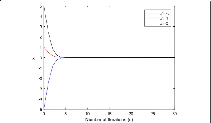
Case 1. Taking the diﬀerent initial pointx1= –5, 1, 5 withη= 1,r= 4, Fig.1presents the

[image:21.595.118.478.498.708.2]

convergence behaviors of{xn}for Algorithm3.1.

(22)

[image:22.595.118.478.91.461.2] [image:22.595.116.477.251.546.2]

Figure 2Behaviors of{xn}with diﬀerentr= 4, 0.4, 0.04,x1= 1 andη= 1

Figure 3Behaviors of{xn}with diﬀerentη= 1, 10, 50, 100, 200,x1= 1 andr= 4

Case 2. Taking the diﬀerentr= 4, 0.4, 0.04 withx1= 1,η= 1, Fig.2presents the

conver-gence behaviors of{xn}for Algorithm3.1.

Case 3. Taking the diﬀerentη= 1, 10, 50, 100, 200 withx1= 1,r= 4, Fig.3presents the

Example4.2 We consider the case thatN1=N2=N3= 2.

LetH1=H2=R,C=Q= [–20, 10] and letfi,hi:C×C→RandFi,Hi:Q×Q→Rbe

deﬁned byf1(z,y) =y2+ 3zy– 4z2,h1(z,y) =y2–z2,F1(z,y) = 3y2+ 2zy– 5z2,H1(z,y) = 0 and f2(z,y) =y2_–_z2_,_h2₍_z_,_y_{) = 0,}_F2₍_z_,_y_{) =}_y2_{+ 3}_zy_{– 4}_z2_,_H2₍_z_,_y_{) =}1

(23)

[image:23.595.119.478.80.308.2]

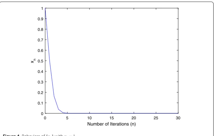
Figure 4Behaviors of{xn}withx1= 1

L,αn,βn,1,ξn,1,λn,γ be the same as that of Example4.1, and deﬁneS2,A2,B2byS2x=4₅x,

A2x= 2xandB2x= 2x. Putβn,2=₂1–_n1₊₂,ξn,2=1₂(1 – _n1₊₁),νn,1=1₂ –_n₊₂1 ,νn,2=1₂+_n₊₂1 , rn,1=rn,2=r= 4,μ1=μ2=1₂andη= 1. It is easy to verify that they satisfy all the conditions

of Theorem3.1.

Following an argument similar to that of Example 4.1, we obtain Trf1,h1(x) = ₁₊₇x_r,

TrF1,H1(x) = ₁₊₈x_r,Trf2,h2(x) = ₁₊₂x_r andTrF2,H2(x) = ₁₊₆x_r andΓ ={0}. Figure4presents the

5 Conclusion

In this paper, we first propose a new parallel hybrid viscosity method for finding a common element of the set of solutions of a finite family of split generalized equilibrium problems, variational inequality problems and the set of common fixed points of a finite family of demicontractive operators in Hilbert spaces. And then we establish the corresponding strong convergence theorem under suitable conditions. We study more general split

equi-librium problems and ﬁxed point problems of operators than those in [18]. Our results

in this paper improve and extend many recent results in the literature. Finally, we present numerical examples to demonstrate the eﬀectiveness of our algorithm.

Acknowledgements

The author is most grateful to the referees and the editor for their helpful comments and advice which helped to improve the contents of this paper.

Funding

Not applicable.

Availability of data and materials

All data generated or analysed during this study are included in this published article.

Competing interests

The author declares to have no competing interests.

Authors’ contributions

(24)

Publisher’s Note

Springer Nature remains neutral with regard to jurisdictional claims in published maps and institutional aﬃliations. Received: 27 February 2019 Accepted: 30 May 2019

References

1. Takahashi, W., Wen, C.-F., Yao, J.-C.: The shrinking projection method for a ﬁnite family of demimetric mappings with variational inequality problems in a Hilbert space. Fixed Point Theory19(1), 407–419 (2018)

2. Dehaish, B.B., Qin, X., Latif, A., Bakodah, H.: Weak and strong convergence of algorithms for the sum of two accretive operators with applications. J. Nonlinear Convex Anal.16, 1321–1336 (2015)

3. Qin, X., Cho, S.Y.: Convergence analysis of a monotone projection algorithm in reﬂexive Banach spaces. Acta Math. Sci.37(2), 488–502 (2017)

4. Chang, S.-S., Wen, C.-F., Yao, J.-C.: Common zero point for a ﬁnite family of inclusion problems of accretive mappings in Banach spaces. Optimization67(8), 1183–1196 (2018)

5. Zhao, X., Ng, K.F., Li, C., Yao, J.-C.: Linear regularity and linear convergence of projection-based methods for solving convex feasibility problems. Appl. Math. Optim.78(3), 613–641 (2018)

6. Ansari, Q.H., Babu, F., Yao, J.-C.: Regularization of proximal point algorithms in Hadamard manifolds. J. Fixed Point Theory Appl.21(1), 25 (2019)

7. Halpern, B.: Fixed points of nonexpanding maps. Bull. Am. Math. Soc.73(6), 957–961 (1967)

8. Cho, S.Y., Dehaish, B.B., Qin, X.: Weak convergence of a splitting algorithm in Hilbert spaces. J. Appl. Anal. Comput. 7(2), 427–438 (2017)

9. Cho, S.Y., Qin, X., Yao, J.-C., Yao, Y.: Viscosity approximation splitting methods for monotone and nonexpansive operators in Hilbert spaces. J. Nonlinear Convex Anal.19, 251–264 (2018)

10. Cho, S.Y., Qin, X., Wang, L.: Strong convergence of a splitting algorithm for treating monotone operators. Fixed Point Theory Appl.2014(1), 94 (2014)

11. Zhang, L., Zhao, H., Lv, Y.: A modiﬁed inertial projection and contraction algorithms for quasi-variational inequalities. Appl. Set-Valued Anal. Optim.2019(1), 63–76 (2019)

12. Yao, Y., Liou, Y.-C., Yao, J.-C.: Iterative algorithms for the split variational inequality and ﬁxed point problems under nonlinear transformations. J. Nonlinear Sci. Appl.10(2), 843–854 (2017)

13. Yao, Y., Liou, Y.-C., Yao, J.-C.: Split common ﬁxed point problem for two quasi-pseudo-contractive operators and its algorithm construction. Fixed Point Theory Appl.2015(1), 127 (2015)

14. Yao, Y., Liou, Y.-C., Kang, S.M.: Approach to common elements of variational inequality problems and ﬁxed point problems via a relaxed extragradient method. Comput. Math. Appl.59(11), 3472–3480 (2010)

15. Kazmi, K.R., Rizvi, S.H.: Iterative approximation of a common solution of a split generalized equilibrium problem and a ﬁxed point problem for nonexpansive semigroup. Math. Sci.7(1), 1 (2013)

16. Cianciaruso, F., Marino, G., Muglia, L., Yao, Y.: A hybrid projection algorithm for ﬁnding solutions of mixed equilibrium problem and variational inequality problem. Fixed Point Theory Appl.2010(1), 383740 (2009)

17. Moudaﬁ, A.: Split monotone variational inclusions. J. Optim. Theory Appl.150(2), 275–283 (2011)

18. Majee, P., Nahak, C.: A hybrid viscosity iterative method with averaged mappings for split equilibrium problems and ﬁxed point problems. Numer. Algorithms74(2), 609–635 (2017)

19. Onjai-uea, N., Phuengrattana, W.: On solving split mixed equilibrium problems and ﬁxed point problems of hybrid-type multivalued mappings in Hilbert spaces. J. Inequal. Appl.2017(1), 137 (2017)

20. Sitthithakerngkiet, K., Deepho, J., Martínez-Moreno, J., Kumam, P.: An iterative approximation scheme for solving a split generalized equilibrium, variational inequalities and ﬁxed point problems. Int. J. Comput. Math.94(12), 2373–2395 (2017)

21. Qin, X., Yao, J.-C.: Weak convergence of a Mann-like algorithm for nonexpansive and accretive operators. J. Inequal. Appl.2016(1), 232 (2016)

22. Ram, T., Lal, P., Kim, J.K.: Operator solutions of generalized equilibrium problems in Hausdorﬀ topological vector spaces. Nonlinear Funct. Anal. Appl.24, 61–71 (2019)

23. Qin, X., Yao, J.-C.: Projection splitting algorithms for nonself operators. J. Nonlinear Convex Anal.18(5), 925–935 (2017) 24. Kim, J.K., Salahuddin, S.: Extragradient methods for generalized mixed equilibrium problems and ﬁxed point

problems in Hilbert spaces. Nonlinear Funct. Anal. Appl.22, 693–709 (2017)

25. Qin, X., Petrusel, A., Yao, J.-C.: CQ iterative algorithms for ﬁxed points of nonexpansive mappings and split feasibility problems in Hilbert spaces. J. Nonlinear Convex Anal.19, 157–165 (2018)

26. Goebel, K., Reich, S.: Uniform Convexity, Hyperbolic Geometry, and Nonexpansive Mappings. Dekker, New York (1984) 27. Marino, G., Xu, H.K.: Weak and strong convergence theorems for strictly pseudo-contractions in Hilbert spaces.

J. Math. Anal. Appl.329, 336–349 (2007)

28. Chidume, C.E., Maruster, S.: Iterative methods for the computation of ﬁxed points of demicontractive mappings. J. Comput. Appl. Math.234, 861–882 (2010)

29. Takahashi, W.: Nonlinear Functional Analysis. Fixed Point Theory and Its Applications. Yokohama Publishers, Yokohama (2000)

30. Mahdioui, H., Chadli, O.: On a system of generalized mixed equilibrium problems involving variational-like inequalities in Banach spaces: existence and algorithmic aspects. Adv. Oper. Res.2012, Article ID 843486 (2012) 31. Censor, Y., Elfving, T.: A multiprojection algorithm using Bregman projections in product space. Numer. Algorithms8,

221–239 (1994)

32. Katchang, P., Kumam, P.: A new iterative algorithm of solution for equilibrium problems, variational inequalities and ﬁxed point problems in a Hilbert space. J. Appl. Math. Comput.32(1), 19–38 (2010)

33. Wang, S., Gong, X., Abdou, A.A., Cho, Y.J.: Iterative algorithm for a family of split equilibrium problems and ﬁxed point problems in Hilbert spaces with applications. Fixed Point Theory Appl.2016(1), 4 (2016)

34. Marino, G., Xu, H.K.: A general iterative method for nonexpansive mappings in Hilbert spaces. J. Math. Anal. Appl.318, 43–52 (2006)

(25)

36. Zegeye, H., Shahzad, N.: Convergence of manns type iteration method for generalized asymptotically nonexpansive mappings. Comput. Math. Appl.62, 4007–4014 (2011)

37. Maingé, P.E.: A hybrid extragradient-viscosity method for monotone operators and ﬁxed point problems. SIAM J. Control Optim.47, 1499–1515 (2008)