DETECTION OF ARRHYTHMIA USING AUTOMATIC DIFFERENTIATION METHOD

(1)

© Associated Asia Research Foundation (AARF)

A Monthly Double-Blind Peer Reviewed Refereed Open Access International e-Journal - Included in the International Serial Directories.

Page | 9

DETECTION OF ARRHYTHMIA USING AUTOMATIC

DIFFERENTIATION METHOD

Shruti Jain

Department of Electronics and Communication Engineering, Jaypee University of Information Technology, Solan

ABSTRACT

ECG records the electrical activity with the help of electrodes placed on different leads and

chest leads. There are different types of leads consisting of unipolar leads, bipolar lead, and

chest lead which form 12 lead system. In this paper pre-processing was done on the data

available from MIT arrhythmia. Different features are extracted using the db4 wavelet with 4

levels. Out of 28 features, best 15 features are selected using Particle swarm optimization

algorithm. Lastly, Back Propagation algorithm is used for the classification where best

performance analysis graph is plotted among Epochs and cross entropy.

Keywords : Electrocardiography, Arrhythmia, Neural Network, Back Propagation, Particle

Swarm Optimization

I. Introduction :

Electrocardiography is the method of recording the electrical activity using electrodes placed

on the skin [1, 2]. These electrodes observe the electro physical pattern of repolarising and

depolarizing of every heart beat. For the normal beat, in Sinoatrial Node (SA) node, electrical

activity associated with each cardiac cycle generates in a cell in right atrium. SA Nodal cells

spontaneously depolarize at a rate that is dependent on the relative balance of sympathetic

and parasympathetic tone [3, 4, 5]. From SA node the wave of depolarization propagates in

an orderly timed fashion to the remaining atrial tissue, to the Atrioventricular Node (AV International Research Journal of Natural and Applied Sciences

ISSN: (2349-4077) Impact Factor- 5.46, Volume 5, Issue 7, July 2018

Website- www.aarf.asia, Email : [email protected] , [email protected]

(2)

Page | 10

Node), then to the left and right ventricular myocardium [6, 7]. The AV node conducts

relatively slowly, thereby allowing the atrium to fully contract before ventricular contraction

starts. At rest, vagal (parasympathetic) tone predominates and the SA node spontaneously

depolarizes, on average, 60-100 times per minute. During exercise, there is both increase in

sympathetic nervous system activity and withdrawal of vagal tone and the SA node may

depolarize at a much faster rate, depending on age [7, 8].

This paper stresses on the analysis of ECG signal which includes four steps [8 – 16] :

denoising, feature extraction [10, 11, 12], feature selection and classifier block [13 - 16].

Section 2 is materials and methods which explain feature extraction of an ECG signal using

different transform techniques, feature selections by best optimization technique (PSO) and

classification using different classifiers. Section 3 explains the results and discussions in

which different parameters/features were extracted using best wavelet technique out of which

best parameters were selected using PSO and Algorithm decomposition is used as the

classifier.

II. Materials and Methods

Before starting with the feature extraction block we have done pre-processing where removal

of the high-frequency noise (power line interference and muscle contraction) is done [4, 5].

2.1Feature Extraction of an ECG signal: When we record ECG signal then it contains a lot

of noise and artifacts present in it so its quality gets degrade and making exact

interpretation of a signal is more difficult. There are mainly two types of FE techniques:

Morphological features (MF) and Signal processing features (SPF) [ 8, 9]

a)Morphological Feature: Morphological image processing could be an assortment of

non-linear operations associated with the morphology of options in a picture.

Morphological operations lies on the relative ordering of pixel values, not on their

numerical values, and thus are particularly suited to the process of binary pictures.

Morphological operations can even be applied to grey scale pictures such their

light-weight transfer functions are unknown and thus their absolute element values are of no

(3)

Page | 11

known as a structuring component. The structuring component is positioned the least

bit attainable locations within the image and it is compared with the corresponding

neighborhood of pixels.

b)Signal Processing Methods: Signal process issues the analysis, synthesis, and

modification of signals that are generally outlined as functions conveyance, signal

process techniques are used to improve signal transmission fidelity, and subjective

quality, and to emphasize or observe parts of interest in a various measured signal. This

is further classified as

i) Fast Fourier Transform: A Fast Fourier Transform (FFT) rule computes the separate

Fourier transform of a sequence, or its inverse (IFFT). An earlier technique used for

analysis of EKG is in time domain, however, this methodology is not comfy for study

all characteristics of ECG signal. So a replacement technique FFT was developed.

Fourier transform might be a regular technique that transforms time domain signal to

the frequency domain to induce the frequency coefficients. The whole method

consists of the subsequent steps: (i) To get an ECG sample as an input signal, (ii)

Compress the ECG input signal by removing the low-frequency components and (iii)

to obtain the original signal by using IFFT. But the disadvantage of FFT is it failed to

provide the information regarding the accurate location of frequency components in

time.

ii)Short Time Fourier Transform (STFT): It is related to a Fourier transform which is

used to determine the sinusoidal frequency and phasor content of a local section of a

signal as it varies with a time. To overcome the problem of an FFT a technique called

the windowed-Fourier transform, i.e. STFT far-famed later as Gabor transform was

introduced. STFT compares both time and frequency information. The STFT is a

quick and straightforward technique compared to other time-frequency analysis. A

window operation is applied to a section of knowledge followed by Fourier

Transform. This can be referred to as the spectrograph or STFT. For a sign x (t), the

definition of STFT is given by the equation.

(4)

Page | 12

STFT {x (t )}(a, w)= X (a, w)=∫ x (t) w (t-a) dt (1)

where w(t) is a window, having duration T, centred at time location t, the Fourier

transform of the windowed signal x(t) w(t - a) is the STFT. But the limitation of STFT

is that its time-frequency precision is not optimal. Hence a more suitable technique is

opted to overcome this drawback known as Wavelet Transform.

iii)Wavelet Transform: Wavelet transform decomposes the signal into the reciprocally

orthogonal set of wavelets that is the main distinction from the continuous wavelet

transform (CWT), or its implementation for the separate statistic generally referred to

as discrete-time continuous wavelet transform (DT-CWT). Hence to beat the matter of

STFT that have mounted window size, therefore, it doesn't provide multi-resolution

information of the signal. However, wavelet transform contains a multi-resolution that

offers each time and frequency information of signal by the variable window size. A

rippling could be a little wave that has energy focused in time and provides a tool for

the analysis of transient, non- stationary or time-varying signals. There are different

types of wavelets: Biorthogonal, Haar, Coiflet, Symlet, Daubechies wavelets, etc. The

wavelet transform may be a time-scale illustration that has been used effectively in an

exceeding type of applications, especially signal compression. It may be a linear

method that decomposes the signal into the variety of scales related to Frequency

elements and analyzes every scale with an explicit resolution.

2.2 Feature Selection (Particle swarm optimization) : Particle swarm optimization

(PSO) is a metaheuristic global optimization method/ stochastic algorithm used for

optimization problem which was put forward originally by Doctor Kennedy and E

Eberhart in 1995. PSO is an evolutionary computation method similar to the Genetic

Algorithm (GA). It is based on the movement of bird and fish flock while searching for

food. The birds can easily smell the food when they are together or scattered, having the

better food resource information, yielding better development of the solution of swarm.

Better the information, optimistic will be its solution which can be worked out with PSO

algorithm. We can also work with complex optimistic problem with PSO. Simplicity and

easier implementation of PSO makes use of this algorithm in many fields such as the

(5)

Page | 13

neural network training, vague system control, automatic adaptation control and machine

learning etc. Many machine learning and deep learning algorithms can be applied to the

classification of Bioinformatics, cyst problem of uterus, cancer of kidney/ lung etc. There

are many other advantages of PSO. They are robust and fast in solving nonlinear,

non-differentiable and multi-modal problems. PSO can be applied into both engineering and

scientific research. PSO adopts real number code. The search can be carried out by the

speed of the particle. Non-linear programming can be easily done with PSO. After so

many advantages of PSO there are some disadvantages as it stuck in the local minima.

To improve the performance of PSO, the researchers proposed the different variants of

PSO. Some researchers try to improve it by improving initialization of the swarm. Some

of them introduce the new parameters like constriction coefficient and inertia weight.

Some researchers work on the global and local best particles by introducing the mutation

operators in the PSO. It has two approaches: one is called cognitive and another is called

social. The particles change its condition according to the three principles: (i) to change

the condition according to its most optimist position (pbest) (ii) to keep its inertia (iii) to

change the condition according to the swarm‘s most optimist position (gbest). The

position of each particle in the swarm is affected by the position of the most optimist

particle in its surrounding (near experience) and the most optimist position during its

movement (individual experience). In the partial PSO, the speed and position of each

particle change according to the equality expression in Eq. (2) and Eq. (3).









1

1 1 2 2

k k k k k k k k

id id id id d id

v  v c r pbest x c r gbest x

(2)

1 1

k k k

id id id

x  x v  ₍₃₎

where v is the velocity, x is the speed of the particle i for k time in the d- dimension of

position. In order to avoid particle being far away from the searching space, the speed of the

particle created at its each direction is confined by vdmax (if the number of vdmax is too small,

the solution will be the local optimism, if the number vdmax is too big, the solution is far from

the best), c1 and c2 represent the speeding figure (if the figure is too small, the particle is

probably far away from the target field, if the figure is too big, the particle will maybe fly to

the target field suddenly or fly beyond the target field). The proper figures for c1 and c2 can

(6)

Page | 14

Usually, c1 is equal to c2 and equal to 2; r1 and r2 represent random fiction. Using Eq. (2)

particle evolution is divided into three parts: better, general and worse.

For better particles position evolution :





1

1 1

k k k k k

id id id id

v  v c r pbest x

(4)

For general particles position evolution









1

1 1 2 2

k k k k k k k k

id id id id d id

v  v c r pbest x c r gbest x

(5)

For worse particles position evolution





1

2 2

k k k k k

id id d id

v  v c r gbest x

(6)

Let‘s consider fmin as the best fitness value, fmax as worse fitness value and aver as the average

value of all fitness. The particles between fmin and aver1 is expressed by Eq. (4) , aver1 and

aver2 is expressed by Eq. (5), aver2 and fmax are expressed by Eq. (6) are known as better

particles, general particles, and worse particles respectively.

2.3 Classification: Classification is the method of grouping the testing samples into the

corresponding categories. Classification is characterized into two varieties viz.

supervised classification and unsupervised classification. MIN-MAX normalization

procedure is used to normalize the extracted and selected features in the range [0, 1] in

order to avoid any bias by unbalanced features. There are various classification

techniques which classify the data into two classes or three classes according to its use.

a) k-Nearest-Neighbour Algorithm (k-NN): The k-NN rule measures the gap between a

question situation and a group of eventualities within the information set.

b) Artificial Neural Network (ANN): An artificial neural network is an interconnected

cluster of nodes, resembling the huge network of neurons of brain. An important

application of neural networks is pattern recognition. Once the network is employed,

it identifies the input pattern and tries to output the associated output pattern. The

ability of neural networks involves once a pattern that has no output related to it, is

given as an input. The system performance is sometimes quantified by means that of

two parameters: sensitivity and specificity or sensitivity and positive prognosticative

accuracy (PPA), once the definition of false negatives could also be questionable.

(7)

Page | 15

speed of true negative events for class, PPA finds the rate of true positive events

among all the classified events in class. There are various neural networks.

I. Feedforward Neural Network : Artificial Neuron: In this type of neural network

the information propagates only in one direction. The information is passed from

the input nodes to the output nodes. This type of neural network might or might

not have the hidden layers of neurons. In straightforward words, it is a front

propagated wave and no backpropagation by employing a classifying activation

operates sometimes.

II. Radial Basis Function Neural Network : RBF functions have 2 layers, initial

wherever the features are combined with the RB operate within the inner layer and

the output of those features are taken into consideration whereas computing an

equivalent output within the next time-step that uses large memory size. The

model depends on the most reach or the radius of the circle in classifying the

points into completely different classes. If the purpose is in or around the radius,

the chance of the new purpose begins categorized into that class is high. The gap

can be measured by Euclidean distance.

III. Kohonen Self Organizing Neural Network: It consists of one or 2 dimensions.

Once training the map the situation of the nerve cell remains constant however the

weights disagree reckoning on the worth. Each nerve cell price is initialized with a

tiny low weight and also the input vector. The nerve cell nearest to the purpose is

that the ‗winning vegetative cell‘ and also the neurons connected to the winning

neuron will move, the space between the purpose and also the neurons is

calculated by the geometer distance, the nerve cell with the smallest amount

distance wins. Through the iterations, all the points are clustered every nerve cell

represents quite cluster.

IV. Recurrent Neural Network(RNN) – Long Short-Term Memory: The RNN works

on the principle of saving the output of a layer and feeding this back to the input

to assist in predicting the end result of the layer. Here, the primary layer is made

like the feed forward neural network with the merchandise of the total of the

weights. The RNN method starts once this is often computed; this implies that

from just the one step to future every nerve cell can bear in mind some data it had

(8)

Page | 16

cell in playing computations. During this method, we want to let the neural

network to figure on the front propagation and bear in mind what data it desires

for later use. Here, if the prediction is wrong we have a tendency to use the

educational rate or error correction to create tiny changes so it'll step by step work

towards creating the proper prediction throughout the backpropagation.

V. Convolutional Neural Network (Conv Net): Convolutional neural networks are the

same as feedforward neural networks,wherever the neurons have learn-able

weights and biases. During this neural network, the input options are taken in

batch wise sort of a filter. This may facilitate the network to recollect the pictures

in components and might work out the operations. These computations involve the

conversion of the image from RGB or IHS scale to Gray-scale. Once we have this,

the changes within the component may be classified into completely different

classes. ConvNet has applied in techniques like signal process and image

classification techniques. PC vision techniques are dominated by ConvNet

attributable to their accuracy in image classification. The technique of image

analysis and recognition, wherever the agriculture and weather options square

measure extracted from the open supply satellites like LSAT to predict the longer

term growth and yield of a specific land are being enforced.

VI. Modular Neural Network: Modular Neural Networks are an assortment of various

networks operating severally and contributory towards the output shown in Fig 1.

Every neural network encompasses a set of inputs that are distinctive compared to

alternative networks constructing and acting sub-tasks. These networks don't act

or signal one another in accomplishing the tasks. The advantage of a modular

neural network is that it breakdowns an outsized computational method into

smaller parts decreasing the complexness. This breakdown can facilitate in

decreasing the quantity of connections and negates the interaction of those

networks with ones another, that successively can increase the computation

speed. However, the interval can rely on the number of neurons and their

(9)

Page | 17

Fig1: Modular Neural Network

VII. Fuzzy hybrid neural network :A fuzzy neural network or neuro-fuzzy system is a

learning machine that finds the parameters of a fuzzysystem

(i.e., fuzzy sets, fuzzy rules) by exploiting approximation techniques from neural

networks. The rule base of a fuzzy system is taken as a neural network. Fuzzy

sets considered weights whereas the input and output variables and therefore the

rules or sculptural as neurons. Neurons is enclosed or deleted within the learning

step. Finally, the neurons of the network represent the fuzzy object.

c) Support Vector Machines (SVM): SVMs have supervised learning models with

associated learning algorithms that analyze knowledge used for classification and

multivariate analysis. SVMs will expeditiously perform a non-linear classification

victimization what's known as the kernel trick, implicitly mapping their inputs into

high-dimensional feature areas When information doesn't seem to be tagged,

supervised learning isn't potential, and an unattended learning approach is needed,

that makes an attempt to seek out natural agglomeration of the information to teams,

so map new information to those shaped teams. The agglomeration rule that provides

Associate in Nursing improvement to the support vector machines is termed support

vector agglomeration and is usually employed in industrial applications either once

information doesn't seem to be tagged or tagged as a preprocessing for a

classification.

d) Back-Propagation: Backpropagation Neural network has two phases. In first phase

training is provided to network‘s input layer. The network propagates the input from

layer to layer until the output pattern is generated by output layer. In the second

(10)

Page | 18

propagated backward from output layer to input layer. Then weights are modified as

the error is propagated. Backpropagation may be a special case of an older and

additional general technique known as Automatic Differentiation. Within the context

of learning, backpropagation is usually utilized by the gradient descent optimization

rule to regulate a load of neurons by shrewd the gradient of the loss operate. This

method is generally known as the backward propagation of errors, as a result of the

error is calculated at the output and distributed back through the network layers.

Backpropagation needs a notable, desired output for every input value—it is so

thought of to be a supervised learning methodology. Backpropagation is additionally a

generalization of the delta rule to multi-layered feedforward networks. It is closely

associated with the Gauss-Newton rule and is an element of continuous analysis in

neural backpropagation. Backpropagation will be used with any gradient-based

optimizer, like L-BFGS or truncated Newton

3 RESULTS and DISCUSSIONS:

We have used Physio BIT MIH database for Arrhythmia patients. Initially pre-processing is

done to remove the noise present in the signal. Out of different FE techniques discussed in

section 2.1 we have used wavelet transform in this paper. Discrete wavelet transforms

method where we discarded the first detail component. The output from denoising block is

passed through low pass and high pass filters. The output of low pass filter is further passed

until enough decomposition is reached. The output of each filter is down sampled by factor 2.

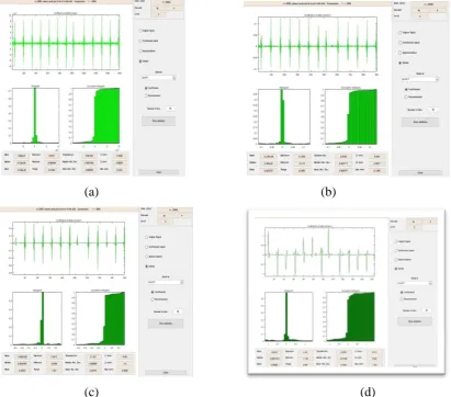
The extraction centered through R-peaks of ECG signal. Fig 2 shows the detail coefficient of

level 4. Here we can see that noise is still at level 3 as ECG signal is not clear enough. Noise

has been removed at level 4, now ECG signal can be analyzed and different features of the

(11)

Page | 19

(a) (b)

[image:11.595.103.515.37.399.2]

(c) (d)

Fig 2 : Detail Coefficient of signal (a) at level 1 (b) at level 2 (c) at level 3 (d) at level

4.

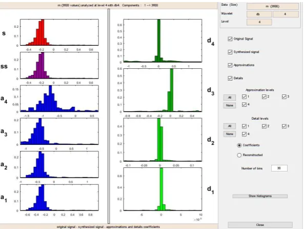
Fig. 3 shows the histogram of signal at level 4. From histogram we can infer that as noise is

removed from level to level histograms of approximation coefficients start expanding. While

the detail coefficient‘s histogram starts shrinking. Synthesized signal has been obtained by

(12)

Page | 20

Fig 3 :Histogram at different levels.

[image:12.595.151.449.34.257.2]

(13)

[image:13.595.177.429.37.222.2]

Page | 21

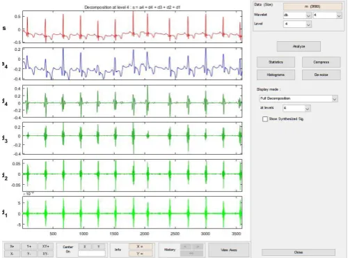
Fig. 5 : decomposition of signal at different levels.

For Feature Extraction, we have chosen db4 wavelet at level 4.While selecting a wavelet for

feature extraction we should keep in mind that wavelet should match with our signal. The

closer the wavelet matches with the signal the better and accurate will be the results. Here

db4 wavelet best match with the ECG signal and at level 4 as a level below 4 we are not able

to get the complete details of the signal whereas above level 4 signals starts deteriorating, so

level 4 is the best where we can get all the details of the signal in Fig 5. d4 refers to the

details coefficient at level 4 and a4 refers to the approximation coefficient at level 4. As we

can see at level 1 detail coefficient contain some noises which are removed further at level 4.

Various features Mean, Median, Standard deviation, Variance, Kurtosis, Skewness,

root-mean-square error (RMSE) and the combination of features with each other were extracted

for 95 images. Out of 28 features, the best features were selected using PSO algorithm. Using

MATLAB 2013a we get, 15 features are the best suites for further computation.

Later the data is divided into testing and training dataset. Confusion Matrix (CM) is used to

outline the performance of a classification model on a particular set of data provided to the

classification model. In CM

a) True Positives (TP): These are the cases in which we forecasted 1(they have an arrhythmia

).

b) True Negatives (TN): These are the cases in which we forecasted 0 (they do not have an

arrhythmia).

c) False Positives (FP): We forecasted 1 and actually they do not have an arrhythmia.

(14)

Page | 22

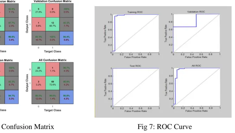
Fig 6: Confusion Matrix Fig 7: ROC Curve

Results we obtained after Training Validating and Testing shows that out of 95 Samples we

were able to predict correctly 22 samples which do not have arrhythmia & 69 samples which

have an arrhythmia. Also in 4 samples, our predictions turn out to be wrong. For training data

set classifier block made a total of 58 predictions. Out of 58, these predictions classifier block

is able to predict that 43 samples have arrhythmia present whereas 13 samples do not have

arrhythmia present shown in Fig. 6. Overall we achieved 95.8% accuracy in predicting

arrhythmia with a 4.2% error rate. From ROC curve (shown in Fig 7) and histogram we can

interpret that at a certain point neural network is unable to predict right response and if we

remove this point from the data set neural network can learn more efficiently. The true

positive rate of a confusion matrix is plotted against the function false positive rate. A ROC

curve reflects the efficiency of a neural network. As we can see in ALL ROC curve which

includes a combined result of Training, Validation, and Testing shown in Fig 7.The graph lies

towards True Positive rate more as we have achieved an overall success rate of 95.8%. An

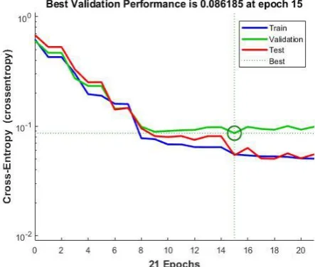
epoch describes the number of times the algorithm sees the entire data set. So, each time the

algorithm has seen all samples in the dataset, an epoch has completed. As we can see that at

[image:14.595.137.518.46.262.2]

(15)

[image:15.595.180.402.42.230.2]

Page | 23

Fig 8: Performance Analysis Graph

CONCLUSION

ECG signal has been through the pre processing block where the different type of noises i.e.

baseline wandering noise, power line interference, burst noise is removed. Then the pre

processed signal is passed through the feature extraction block from where different features

of signal i.e. mean, median, kurtosis, skewness, variance, standard-deviation, rmse are

extracted. In classification block data set is provided for ECG signal classification. Their

using Backpropagation neural network algorithm training, validation, and testing are

performed. From the classifier block, we have achieved a 95.8% accuracy in predicting the

arrhythmia along with a 4.2% error rate which is shown in the confusion matrix.

References

1. Carr J. J., John M.Brown,‖Introduction to Biomedical Equipment Technology‖.

2. Thakor N.V., ―Electrocardiographic monitors,‖ in Encyclopedia of Medical Devices

and Instrumentation,

3. John G. Webster, Halit Eren. ,‖Measurement, Instrumentation and Sensors

Handbook‖.

4. Prashar N. et al, "Removal of electromyography noise from ECG for high

performance biomedical systems," Network Biology, vol. 8, p. 12, 2018.

5. Prashar N. et al, ―Review of Biomedical System for High Performance Applications‖,

4th IEEE International Conference on signal processing and control (ISPCC 2017), Jaypee University of Information technology, Waknaghat, Solan, H.P, India, pp

(16)

Page | 24

6. Ishbeata A, Kalbouneh M. ―ECG Circuit Analysis and Design‖: Jan 11, 2012

7. Gupta R., Singh S., Garg K., Jain S., ―Indigenous Design of Electronic Circuit for

Electrocardiograph‖, International Journal of Innovative Research in Science,

Engineering and Technology, 3(5), 12138-12145, May 2014

8. Dhiman A, Singh A, Dubey S, Jain S., “Design of Lead II ECG Waveform and

Classification Performance for Morphological features using Different Classifiers on

Lead II ”, Research Journal of Pharmaceutical, Biological and Chemical Sciences

(RJPBCS),7(4), 1226- 1231: July-Aug 2016.

9. Jain S., "Classification of Mitogen Activated Protein Kinase using Different Wavelet

Transforms (Discrete and Gabor)," Asian Journal of Microbiology, Biotechnology

and Environmental Sciences, vol. 20, pp. 569-574, 2018.

10.Jain S., "Classification of Protein Kinase B using discrete wavelet transform,"

International Journal of Information Technology, vol. 10, pp. 211-216, 2018.

11.Bhusri S., Jain S., Virmani J., "Breast Lesions Classification using the Amalagation of

morphological and texture features," International Journal of Pharma and

BioSciences, vol. 7, pp. 617-624, 2016.

12.Rana S., Jain S., Virmani J., "Classification of focal kidney lesions using

wavelet-based texture descriptors," International Journal of Pharma and Bio Sciences, vol. 7,

pp. 646-652, 2016.

13.Bhusri S., Jain S., Virmani J., "Classification of breast lesions using the difference of

statistical features," Research Journal of Pharmaceutical Biological And Chemical

Sciences, vol. 7, pp. 1365-1372, 2016.

14.Sharma S., Jain S., Bhusri S., " Two Class Classification of Breast Lesions using

Statistical and Transform Domain features," Journal Of Global Pharma Technology

Methodology, vol. 9, pp. 18-24, 2017.

15.Jain S, Bhooshan S.V., Naik P.K., ―Mathematical modeling deciphering balance

between cell survival and cell death using insulin‖, Network Biology, 1(1):46-58,

2011.

16.Afkhami R. G., Azarnia G., Tinati M. A., "Cardiac arrhythmia classification using

statistical and mixture modeling features of ECG signals," Pattern Recognition

Letters, vol. 70, pp. 45-51, 2016.