http://dx.doi.org/10.4236/opj.2014.41001
Vortex Field Propagation in a Hexagonal
Multicore Fiber Array
Muhammad A. Mushref
Department of Electrical Engineering and Computer Science, University of Wisconsin-Milwaukee, Milwaukee, USA
Email: [email protected], [email protected]
Received November 22, 2013; revised December 17, 2013; accepted January 5, 2014
Copyright © 2014 Muhammad A. Mushref. This is an open access article distributed under the Creative Commons Attribution Li-cense, which permits unrestricted use, distribution, and reproduction in any medium, provided the original work is properly cited. In accordance of the Creative Commons Attribution License all Copyrights © 2014 are reserved for SCIRP and the owner of the intel-lectual property Muhammad A. Mushref. All Copyright © 2014 are guarded by law and by SCIRP as a guardian.
ABSTRACT
The propagation of an optical vortex in a hexagonally arranged single mode multicore fiber structure is investi- gated for possible generation of additional vortices and their spread dynamics. Fields are separated into a slowly varying paraxial envelope and a rapidly changing exponential component. Solutions are derived from the par- axial inhomogeneous Schrodinger equation in two dimensions along with the index of refraction of the proposed structure. Numerical analyses are based on the beam propagation method and transparent boundary conditions in matrix form with different parameters to represent the intensity and phase of all derived fields. Vortices are numerically identified by their points of zero intensity and their phase change or polarity. The optical interfero- gram with a plane wave reference is also employed to distinguish the dislocation points in the transverse direc- tions of the propagating fields.
KEYWORDS
Optical Vortex; Beam Propagation Method; Transparent Boundary Conditions; Multicore Fibers; Optical Interferogram
1. Introduction
The propagation of light and its waveguiding properties in periodic lattices or multicore fibers is one of the im-portant fields of study in photonics. Optical vortices tra-velling in such structures form a very rich area of re-search due to their intensity and phase features. The sig-nificant implication is their possible attractive applica-tions in optical switching, modulation and sensing [1,2]. There are several theoretical and experimental published studies in the literature that examined the propagation of optical vortices and their overall behavior. Though, pre-vious investigations did not verify possible relations be-tween newly generated vortices and the propagation dis-tance with the effects of different parameters such as structure size and number of cores.
Dispersion and size of guided beams are numerically determined for an optical vortex soliton in a graded index waveguide [3]. The propagation of a stationary pulse in circularly arranged coupled cores is also numerically
lattices, single charge vortices are found to exhibit dyna- mical instabilities and thus their breakup occurs at short propagation distances compared to double charge vortic- es [12].
2. Formulation and Method
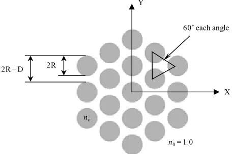
The relation between the generated optical vortices in a multicore fiber and the propagation distance is yet to be explored. In this paper, the propagation of an optical vortex in a multicore fiber is theoretically and numeri- cally investigated. All cores are assumed single mode and identical such that they are of equal radius in a hex- agonal arrangement with equal distances from each other and with the same index of refraction in a step profile. An example for the proposed structure is shown in Fig- ure 1 for 19 cores in a normalized rectangular coordi-nates as X = x/w0 and Y = y/w0 with a normalized ra- dius of each core as R = r/w0 and a normalized dis- tance between cores as D = d/w0 where w0 is the beam width and r and d are in μm. The index of refraction of each core is assumed very close to that of free space with
a difference of 0 approximately
where n0 = 1.0 for free space. Beam propagation method (BPM) with transparent boundary conditions (TBC) are employed to solve for the propagating optical vortex beam in the proposed multicore fiber [13-15]. Different parameters are also considered in the solutions such as number of cores, core size and their distances from each other.
Δ 0 005
c
n n n .
The solutions start from the source-free Maxwell’s equations to find the Helmholtz scalar wave equation for the field ψ(x, y, z) in the rectangular coordinate system as where n(x, y) is the refractive index of the medium. In beam propagation method, backward waves are ignored and the fields are separated as a paraxial slowly varying envelope (x, y, z) multi-plied by a rapidly varying exponential part in the form
2 2 20 0
k n x, y
X Y
2R 2R + D
n0= 1.0
nc
[image:2.595.57.285.558.709.2]60˚ each angle
Figure 1. Schematic transverse section of the proposed
[16]:
x y z, ,
x y z e, ,
jk n z0 0 (1) where n0 and k0 are the free space index of refraction and
(1) in the Helmholtz scalar w
wavenumber respectively. By substituting Equation
ave equation, the propagation of the optical field can be described by the inhomogeneous normalized Schrodinger equation in the form [15]:
2 T
2 2 2 2
0 0 0
Φ X,Y,Z
Φ X,Y,Z 4
Z
X,Y Φ X,Y,Z 0
j
k w n n
(2)
where, 2 2 2 2
T X Y
2
,Φ(X, Y, Z) is the nor- paraxial slowly varyin
lved for the field Φ(X, Y,
1
malized g field envelope, n (X,Y)
is the structure refractive index, Z = z/z0, z0 = πw02/λ and
λ is the wavelength.
3. Numerical Analyses
Equation (2) is numerically soZ) using finite difference (FD) and split-step techniques by employing the calculation steps of X = Xm= mΔX, Y
= Yp = pΔY and Z = Zq= qΔZ [16]. Calculation steps are
assumed as m = 1, 2, 3, ···, M, p = 1, 2, 3, ···, P and q = 1, 2, 3, ···, Q, where M and P are the transverse field reso-lution with an assumption of M = P = N. Also, Q is the number of longitudinal steps in Z which is the direction of field propagation along the optical waveguide. Thus, Equation (2) can be split to generate two equations in the form:
, 1, 1,
, , 1 ,
Φ Φ Φ
Φ Φ Φ
*q * q *q m p m p m p
q q q
m p m p m p
A C B C
(3a)
1 1 1
, , 1 , 1
ΔZ 4
, 1, 1,
Φ Φ Φ
Φ Φ Φ
q q q
m p m p m p
jT * q * q * q
m p m p m p
A C
B C e
(3b)
where 2 2 2
20 0 X, Y 0
T k w n n
*
is the influence of the ttice material, is a num
Equations (3a) and (3b), th
(4a)
1
N
fiber la erical intermediate
val-ue of the normalized field, A = 1 −α, B = 1 + α, C = α/2,
α= jΔZ/4Δ2 and ΔX = ΔY = Δ. In order to numerically solve ey are transformed to matrix form as:
1 1 1
Φ N N N
N L F
1 1Φ N L N N G (4b) where F and G are the right hand expressions in Equa- tions (3a) and (3b) respectively and L is an N × N tridi-agonal matrix given by:
0 0
0 0
0
0 0 N N
C A C
L C A
C C A
A C
(5)
The transverse distribution of the initial field is as-su
lized optical vortex at Z = 0 can be ex
med to be Φ1 for q = 1 and it is used in Equation (4a) at the beginning of the solution. Once Φ*1 is calculated, it is then used in Equation (4b) to solve for Φ2 which is the field in the next longitudinal step at q = 2. This process is repeated for any required distance in the normalized lon-gitudinal direction.
The initial norma
pressed as a Laguerre-Gaussian mode of the first order given by [17]:
2
[image:3.595.341.504.83.598.2] [image:3.595.118.227.88.159.2]Φ , e j (6) where Φ
,
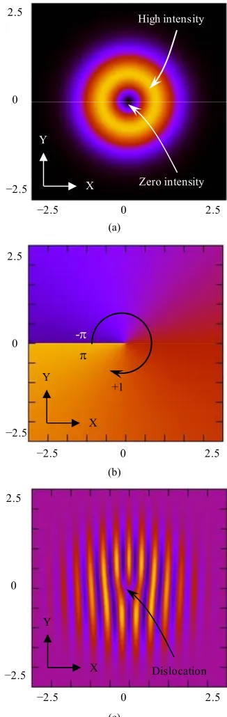
is the vortex optical field, j = 1, ρ2 = X2 + = tan−1 (Y/X).Figure 2 illustrates the initi Y2 and φ
al optical vortex used in th
4. Results and Discussions
e performed for nc =
is paper which is numerically generated for N = 500, Δ = 0.01, w0 = 5 μm and λ =1.5 μm with y = x and x = Xw0 = NΔw0 = 25.0 μm. The field intensity is shown in Fig-
ure 2(a) with the point of zero intensity at the origin and
Figure 2(b) shows the phase change from –π to π. Fig- ure 2(c)is the interferogram with a plane wave reference that shows the point of dislocation with a vortex topo-logical charge or polarity of +1 at the origin.
All analyses and simulations ar
1.005, beam width of w0 = 5.0 μm and wavelength of λ = 1.5 μm with 2
0 π 0
z w 52.36 μm. Single mode cores are assumed with a V number as V 2πrNA 2 405.
where 2 2
0 0 1
c
NA n n . is the numerical aperture. propagated optical v
41
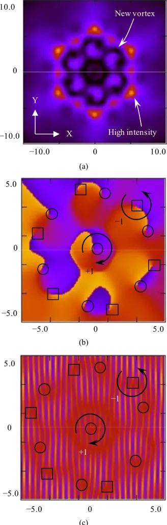
The ortex field at Z = 8 (z = Zz0 = 8.88 μm) is shown in Figure 3for 61 cores with R = 0.4 (r = Rw0 = 2.0 μm), D = 0.2 (d = Dw0 = 1.0 μm), a resolution of N = 1000 and calculation steps of Δ = 0.09 and ΔZ = 0.01. Figure 3(a) is a zoomed in image of the field intensity that illustrates the spots of light in some cores. Since the cores are very close to each other at a constant distance, the field is coupled between them as it propagates. The phase of the field with charges of +1 or −1 of newly generated vortices is shown as a zoomed in image in Figure 3(b) where they demonstrate a phase change from –π to π. The total charge or polarity of vor- tices should be conserved to +1 which is the charge of the initial transmitted vortex field. Topological charge should be always conserved when new optical vortices are formed and then annihilated in pairs with opposing
X Y
Zero intensity
2.5 −2.5
2.5
−2.5
0 0
High intensity
(a)
-
X Y 2.5
−2.5 0
2.5
−2.5 0
+1
(b)
X Y 2.5
−2.5 0
2.5
−2.5 0
Dislocation
(c)
Figure 2. Intensity (a), phas ) and interferogram with a
harges [18]. In this case, conservation is confirmed as 7 e (b
plane wave reference (c) of an optical vortex for N = 500, Δ = 0.01, w0 = 5 μm and λ = 1.5 μm.
c
X Y
10
−10 0
10
−10 0
High intensity
(a)
3.0
−3.0 0
3.0
−3.0 0
+1
−1
(b)
3.0
−3.0 0
3.0
−3.0 0
+1
−1
[image:4.595.91.256.83.602.2](c)
Figure 3. Intensity (a), phas ) and interferogram with a
Moreover, Figure 4 shows the propagated optical vor- te
e (b
plane wave reference (c) of an optical vortex for N = 1000, Δ = 0.09, Z = 8.0, w0 = 5 μm and λ =1.5 μm. = −1 charge and
= +1 charge.
x field at Z = 11 for 127 cores with R = 0.4, D = 0.2, a resolution of N = 1000 and calculation steps of Δ = 0.04 and ΔZ = 0.01. Figure 4(a) is a zoomed in image from −10.0 to 10.0 of the field intensity with the spots of light coupled and spread in more cores compared to the case
X Y
10.0
−10.0 0
10.0
−10.0 0
High intensity New vortex
(a)
5.0
−5.0 0
5.0
−5.0 0
+1 −1
(b)
5.0
−5.0 0
5.0
−5.0 0
+1
−1
[image:4.595.341.505.86.602.2](c)
Figure 4. Intensity (a), phas ) and interferogram with a
Figure 3(a). The phase of the field from –π to π is e (b
plane wave reference (c) of an optical vortex for N = 1000, Δ = 0.04, Z = 11.0, w0 = 5 μm and λ = 1.5 μm. = −1 charge
and = +1 charge. in
re-spect to the X axis that shows the points of dislocations for each created vortex.
The approach discusse
n r is w v d
d in Figures 3 and 4 is employ- ed
Table 1. Generated vortices for different number of cores
Z 37 cores 61 cores 91 cores 127 cores
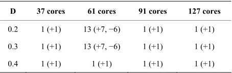
to investigate the generation of new vortices with re-spect to Z when the number of cores, R or D parameters are varied. Results are listed in Table 1 for Z from 0.0 to 20.0 when the number of cores is 37, 61, 91 and 127 re-spectively and visualized in Figure 5 for R = 0.4 and D = 0.2 for the same number of cores. Polarities of new vor-tices are also recorded in Table 1 which clearly demon-strate and confirm the conservation of charge. The curves shown in Figure 5 have meaning only at the data points in Table 1 at integer values for the same parameters. As exposed, the generation of new vortices is very dynamic and highly varied with respect to Z and the number of cores. More vortices are created as the number of cores increases and the beam propagates at farther distances. New vortices start to appear at shorter propagation dis- tance but more new vortices are produced when the
for R = 0.4 and D = 0.2 (polarities are shown between pa-rentheses).
0.0 1 (+1) 1 (+1) 1 (+1) 1 (+1)
1.0 1 (+1) 1 (+1) 1 (+1) 1 (+1)
2.0 1 (+1) 1 (+1) 1 (+1) 1 (+1)
3.0 1 (+1) 1 (+1) 1 (+1) 1 (+1)
4.0 1 (+1) 1 (+1) 1 (+1) 1 (+1)
5.0 1 (+1) 1 (+1) 1 (+1) 1 (+1)
6.0
umbe of cores higher. Ho ever, new ortices coul not exist continually and may possibly vanish with other new vortices generated at different locations.
As in Table 1, the longitudinal distance at Z = 8.0 shows differences in the number of new vortices as the number of cores is varied. Core radius may also affect the number of new generated vortices as listed in Table 2
and visualized in Figure 6 for R = 0.2, 0.3 and 0.4, Z = 8.0 and D = 0.2 for the same number of cores. The gen-eration of new vortices is very sensitive to the core radius when there are more cores such as the sharp change from 1 vortex to 11 vortices and then to 1 vortex for 127 cores. In addition, variation of the distance between cores could show some changes in the number of new vortices as listed in Table 3 and visualized in Figure 7 for D =
Figure 5. Created vortices with respect to Z for different cores for R = 0.4 and D = 0.2.
3
13
3 ) 1
5 )
3
7 )
2
3
(+2, −1) 1 (+1) 1 (+1) 1 (+1)
7.0 1 (+1) (+7, −6) 1 (+1) 1 (+1)
8.0 1 (+1) 13 (+7, −6) (+2, −1 (+1)
9.0 1 (+1) 11 (+6, −5) 13 (+7, −6) 1 (+1)
10.0 1 (+1) 1 (+1) 13 (+7, −6) (+3, −2
11.0 1 (+1) 1 (+1) 15 (+8, −7) 13 (+7, −6)
12.0 1 (+1) 1 (+1) 11 (+6, −5) 13 (+7, −6)
13.0 (+2, −1) 1 (+1) 7 (+4, −3) 13 (+7, −6)
14.0 1 (+1) (+4, −3 3 (+2, −1) 13 (+7, −6)
15.0 1 (+1) 11 (+6, −5) 13 (+7, −6) 13 (+7, −6)
16.0 1 (+1) 13 (+7, −6) 13 (+7, −6) 19 (+10, −9)
17.0 1 (+1) 3 (+12, −11) 13 (+7, −6) 31 (+16, −15)
18.0 1 (+1) 23 (+12, −11) 13 (+7, −6) 33 (+17, −16)
19.0 1 (+1) 17 (+9, −8) 13 (+7, −6) 33 (+17, −16)
20.0 (+2, −1) 13 (+7, −6) 11 (+6, −5) 27 (+14, −13)
Figure 6. Created vortices with respect to R for different
ith core radius R for different
91 cores 127 cores
cores for Z = 8.0 and D = 0.2.
Table 2. Generated vortices w
nu ber of cores for Z = 8.0 and D = 0.2 (polarities are shown between parentheses).
R 37 cores 61 cores
m
0.2 1 (+1) 1 (+1) 1 (+1) 1 (+1)
0.3 1 (+1) 1 (+1) 9 11
13
(+5, −4) (+6, −5)
Figure 7. Created vortices with respect to D for diffe e
th distance D for different
91 cores 127 cores
r nt cores for Z = 8.0 and R = 0.4.
able 3. Generated vortices wi
T
number of cores for Z = 8.0 and R = 0.4 (polarities are shown between parentheses).
D 37 cores 61 cores
0.2 1 (+1) 13 (+7, −6) 1 (+1) 1 (+1)
0.3 1 (+1) 13 (+7, −6) 1 (+1) 1 (+1)
0.4 1 (+1) 1 (+1) 1 (+1) 1 (+1)
.2, 0.3 and 0.4, R = 0.4 and Z = 8.0. This parameter may
clusion
s are presented for the propagation of
REFERENCES
[1] D. N. Christo0
have an increasing effect such as the change of the num- ber of vortices from 1 to 3 in a 37 cores array. Also, it could have a decreasing effect such as the change from 13 to 1 in a 61 cores array or from 3 to 1 in a 91 cores array.
5. Con
Theoretical analyse
an optical vortex field in a single mode multicore fiber array. The derivations employed beam propagation me-thod and transparent boundary conditions to obtain the numerical solutions. Investigations explained the highly dynamical nature of the propagating vortex in the pro- posed structure. Different parameters were examined such as the number of cores and the size of the structure that could have an effect on the creation of new vortices. It is found that vortices are very responsive to variations of the array parameters either by increasing or by de- creasing the number of vortex pairs given that the topo- logical charge is conserved.
doulides, F. Lederer and Y. Silberberg, “Discretizing Light Behavious in Linear and Nonlinear Waveguide Lattices,” Nature, Vol. 424, No. 6950, 2003, pp. 817-823. http://dx.doi.org/10.1038/nature01936 [2] J. Demas, M. D. W. Grogan, T. Alkeskjold and S. Rama-
chandran, “Sensing with Optical Vortices in Photonic- Crystal Fibers,” Optics Letters, Vol. 37, No. 18, 2012, pp. 3768-3770. http://dx.doi.org/10.1364/OL.37.003768 [3] C. Law, X. Zhang and G. Swartzlander Jr., “Waveguiding
Properties of Optical Vortex Solitons,” Optics Letters, Vol. 25, No. 1, 2000, pp. 55-57.
http://dx.doi.org/10.1364/OL.25.000055 [4] A. Buryak and N. Akhmediev, “S
gation in N-Core Nonlinear Fiber Arrays
tationary Pulse Propa- ,” IEEE Journal of Quantum Electronics, Vol. 31, No. 4, 1995, pp. 682- 688. http://dx.doi.org/10.1109/3.371943
[5] J. K. Yang and Z. H. Musslimani, “Fundamental and Vor- tex Solitons in a Two-Dimensional Optical Lattice,” Op- tics Letters, Vol. 28, No. 21, 2003, pp. 2094-2096. http://dx.doi.org/10.1364/OL.28.002094
[6] T. J. Alexander, A. A. Sukhorukov and Y. S. Kiv “Asymmetric Vortex Solitons in Nonline
shar, ar Periodic Lat- tices,” Physical Review Letters, Vol. 93, No. 6, 2004, pp. 63901-63905.
http://dx.doi.org/10.1103/PhysRevLett.93.063901 [7] D. N. Neshev, T
Kivshar, H. Martin, I. Makasyuk and Z. G. Chen . J. Alexander, E. A. Ostrovskaya, Y. S.
, “Ob- servation of Discrete Vortex Solitons in Optically Induc- ed Photonic Lattices,” Physical Review Letters, Vol. 92, No. 12, 2004, pp. 123903-123906.
http://dx.doi.org/10.1103/PhysRevLett.92.123903 [8] Z. G. Chen, H. Martin and A. Bezryad
on Gaussian Beams and Vortices in Optically Induced ina, “Experiments
Photonic Lattices,” Journal of the Optical Society of Ame- rica B, Vol. 22, No. 7, 2005, pp. 1395-1405.
http://dx.doi.org/10.1364/JOSAB.22.001395 [9] M. I. Rodas-Verde and H. Michinel, “Dynamic
Solitons and Vortices in Two-Dimensional P
s of Vector hotonic Lat- tices,” Optics Letters, Vol. 31, No. 5, 2006, pp. 607-609. http://dx.doi.org/10.1364/OL.31.000607
[10] B. Terhalle, T. Richter, A. S. Desyatnikov, D. N. Neshev, W. Krolikowski, F. Kaiser, C. Denz and Y. S. Kivshar, “Observation of Multivortex Solitons in Photonic Lattic- es,” Physical Review Letters, Vol. 101, No. 1, 2008, pp. 13903-13906.
http://dx.doi.org/10.1103/PhysRevLett.101.013903 [11] B. Terhalle, T. R
T. J. Alexander, P. G. Kerekidis, A. S. Desyatniko ichter, K. J. H. Law, D. Gories, P. Rose,
v, W. Krolikowski, F. Kaiser, C. Denz and Y. S. Kivshar, “Ob- servation of Double-Charge Discrete Vortex Solitons in Hexagonal Photonic Lattices,” Physical Review A, Vol. 79, No. 4, 2009, pp. 43821-43829.
http://dx.doi.org/10.1103/PhysRevA.79.043821 [12] K. J. H. Law and P. G. Kevrekidis, “
Discrete Vortices in Hexagonal Optical Lattices
Stable Higher-Charge ,” Physi- cal Review A, Vol. 79, No. 2, 2009, pp. 25801-25805. http://dx.doi.org/10.1103/PhysRevA.79.025801 [13] C.-S. Hsiao, L. Wang and Y. J. Chiang, “An Algorith
for Beam Propagation Method in Matrix Form m ,” IEEE Journal of Quantum Electronics, Vol. 46, No. 3, 2010, pp. 332-339. http://dx.doi.org/10.1109/JQE.2009.2029066 [14] S. A. Shakir, R. A. Motes and R. W. Berdine, “Efficient
[image:6.595.59.286.299.371.2]http://dx.doi.org/10.1109/JQE.2010.2091395
[15] D. Jimenez and F. Perez-Murano, “Improved Boundary Conditions for the Beam Propagation Method,” IE Photonics Technology Letters, Vol. 11, No. 8
EE , 1999, pp. 1000-1002. http://dx.doi.org/10.1109/68.775326
[16] K. Okamoto, “Fundamentals of Optical Waveguides,” Elsevier Inc., Maryland Heights, 2006.
[17] B. Saleh and M. Teich, “Fundamentals of Photonics,”
Duijl and J. P. John Wiley & Sons, Inc., Hoboken, 2007.
[18] G. P. Karman, M. W. Beijersbergen, A. van
Woerdman, “Creation and Annihilation of Phase Singula- rities in a Focal Field,” Optics Letters, Vol. 22, No. 19, 1997, pp. 1503-1505.