Lancaster University Management School
Working Paper
2003/088
On the Errors and Comparison of Vega Estimation Methods
Mark Shackleton and San-Lin Chung
The Department of Accounting and Finance Lancaster University Management School
Lancaster LA1 4YX UK
©Mark Shackleton and San-Lin Chung All rights reserved. Short sections of text, not to exceed two paragraphs, may be quoted without explicit permission,
provided that full acknowledgement is given.
The LUMS Working Papers series can be accessed at http://www.lums.lancs.ac.uk/
On the errors and comparison of Vega estimation
methods.
San-Lin Chung
Department of Finance, National Taiwan University
Mark Shackleton
∗Accounting and Finance, Lancaster University
October 2003
Abstract
This article discusses convergence problems when calculating Vega
(op-tion sensitivity to volatility) that arise from discretiza(op-tion errors embedded
in the lattice approach. Four alternative improvements to the traditional
binomial method are discussed and investigated for performance. We also
propose a new Modified Binomial (MB) Method to calculate Vegas.
Numer-ical results show that although the MB is not the most price accurate of the
models, due to its error structure as a function of volatility, it produces the
most accurate and fastest Vega estimates. JEL: G13. Keywords: Vega,
lattice approach, discretization error, smoothing.
∗Lancaster LA1 4YX, UK. tel 44 (0) 1524 594131, fax 847321. Thanks go to the Editor and
1
Introduction
Once the price of an option position has been negotiated and the position
estab-lished, tracking and maintenance of the hedging properties is an essential task not
only for the buyer but especially for the option seller. This is because the option’s
risk characteristics change dynamically as the stock price and time to maturity
change. Therefore the so called “Greeks” (or partial differentials) with respect to
model variables must be calculated accurately and repeatedly.
For many different option models and numerical estimation methods, there is a
body of literature concerning the properties of these Greeks which recognises that
numerical procedures are problematic. While producing option sensitivities that
converge in the number of time steps (grid points or tree nodes), numerical
dif-ferentiation is hazardous because results converge in an oscillatory fashion (see
Pelsser and Vorst (1994) and Chung and Shackleton (2002) for details).1
As well as the first (second) differentials with respect to price and timevariables,
Delta, (Gamma) and Theta, there are Greeks that represent differentials with
respect to option parameters. The first differential with respect to volatility (and
interest rate), Vega (Rho), are also calculated and often quoted even though many
option models assume these factors to be constant. This is because these are used
in a slightly different, but no less important manner by purchasers and hedgers of
options.
There several reasons why an option’s sensitivity to a fixed (or potentially non—
dynamic) parameter needs to be considered and calculated repeatedly and
accu-rately. It is also clear for option models that explicitly model stochastic volatility
1This is largely due to the fact that changing the number of time steps (or another numerical
paramater) changes the number of nodes either side of the exercise point, therefore the estimated
and treat it as a variable, why Vega sensitivity is important.
Firstly, even if an option model has a fixed volatility, there is the danger of
param-eter mis—estimation. It may be the case that volatility may be constant but just
difficult to estimate accurately with limited data. This means that the sensitivity
of a model’s volatility assumption needs to be examined through its Vega in order
to test the sensitivity to any one particular chosen volatility value.
Secondly, even for constant volatility models, potential uncertainty about the exact
model specification means that different models may be used not only to estimate
the option’s price but also to estimate the impact of the same volatility assumption
in different models.
Thirdly, for tractability, many practitioners may assume that these last two
vari-ables (volatility and interest rates) are known and constant, in the knowledge that
this is only an approximation. If the validity of this assumption is questionable,
they may use two option positions with opposite Vega in an attempt to eliminate
their volatility risk. Essentially they may estimate Vega from each model with
constant volatility, hoping that if volatility actually changes that it will affect both
of the mis—specified model prices to the same degree and due to the supposed Vega
neutrality, cancel each other out.
Finally, there are an increasing number of models that include stochastic rather
than fixed volatility. Although in this paper we apply numerical methods to the
estimation of Vega sensitivity with fixed volatility, its results relate to other more
complex Vega calculation problems.
This article continues in Section 2 with a review of the five methods that are
cur-rently used or discussed in the literature. In Section 3, we propose a new method,
each of the five existing methods as well as the new method proposed. Section 5
examines the root mean square error against computational speed (efficiency) of
each method while Section 6 concludes.
2
Vega estimation
The numerical error of Vega estimates is mainly due to the discretization embedded
in the binomial lattice approach, particularly at option expiry where the positioning
of nodes with respect to the exercise price is critical. Within the literature, there
are at least four proposed solutions that reduce the discretization errors or enhance
the rate of convergence compared to the standard tree structure. Firstly, addition
of one or more small sections of fine high—resolution lattice within a tree with
coarser time and price steps (see Figlewski and Gao (1999)). Secondly, adjustment
of the discrete—time solution prior to maturity (see Broadie and Detemple (1996)
and Heston and Zhou (2000)) or smoothing of the payoffs at maturity (see Heston
and Zhou (2000)). Finally, allocation and number (the shape and span) of tree
nodes (see Ritchken (1995), Tian (1999) and Widdicks, Andricopoulos, Newton,
and Duck (2001)). In this section we review the motivation and construction of
each method.
2.1
Binomial method
In the lattice approach to option pricing and hedging (for example see Hull (2000)),
it is common wisdom in calculating Vega to make a small change, ∆σ, to the
volatility σ and construct a new tree to obtain a new value of the option. This is
then used to calculate a numerical derivative. Since the magnitude of the pricing
well as other things), usually the same number of steps is used so as to minimize
potential errors involved in this numerical differentiation. The estimate of Vega is
then
V (σ,∆σ, n) = P (σ+∆σ, n)−P (σ, n)
∆σ (1)
where P (σ+∆σ, n) and P (σ, n) are the estimates of the option price from the
original and the new tree, respectively (both withnsteps). Note that this is only a
numerical differential of the true sensitivity V (σ,0, n) = lim∆σ→0V (σ,∆σ, n) and
as such will contain estimation error for the Vega that depends on the size of ∆σ
and the number of tree steps (n).
However there is a convergence problem similar to that of pricing barrier—type
op-tions (see Boyle and Lau (1994) and Ritchken (1995)). This method for calculating
Vega also faces discretization errors embedded within the lattice approach,
partic-ularly with respect to the positioning of final nodes around the exercise threshold.
The problem is serious because the two estimates of the option price are obtained
using two different trees where thefinal nodes are non—coincident (i.e. same
num-ber but differently placed nodes) so that discretization errors in each estimate are
imperfectly correlated and do not cancel.
Pest.(σ, n) = Ptrue(σ, n) +ε(σ, n) (2)
Pest.(σ+∆σ, n) = Ptrue(σ+∆σ, n) +ε0(σ+∆σ, n)
V (σ,∆σ, n) = Pest.(σ+∆σ, n)−Pest.(σ, n)
∆σ (3)
= Ptrue(σ+∆σ, n)−Ptrue(σ, n)
∆σ +
ε0(σ+∆σ, n)−ε(σ, n)
∆σ
Thus with imperfectly correlated errors, Vega is always estimated with error. This
total error will depend on the way the second error depends on thefirst. If the best
fit line between them is of unit slope and zero intercept, then their cancellation can
fit between the two errors. Thus investigation of the error dependency is a crucial
part of the analysis of Vega estimation. This is conducted in Section 4.
2.2
Adaptive Mesh Model (AMM)
In order to improve price convergence Figlewski and Gao (1999) propose a method
termed the Adaptive Mesh Model (AMM) to reduce the convexity error at the
terminal boundary. In their method, one or more small sections of fine high—
resolution lattice are added into a tree with coarser time and price steps. This
incorporates a finer mesh of values around the critical nodes in the coarse tree and
thus achieves greater accuracy by reducing the non—linearity error.
This method has been shown to reducepricingerrors considerably. The cost is that
the tree now has different structures in different regions and so is more complex to
implement. Furthermore, although thelocationof the maximum convexity is know
(near the money at maturity), the choice ofspanaround this area is arbitrary. Any
number of extra nodes between two and the number of steps already used could be
added (in the latter case the tree is again a regular one with twice as many steps).
Thus this method partially smooths the option price with respect to a perturbation
of its parameters. With the increased node density around the exercise threshold,
price oscillation innis also reduced. However in light of Equation 2 the correlation
of these errors is shown to be as important as the magnitude and so the correlation
structure of the price errors should also be considered.
As will be seen in Section 4 a lack of error correlation structure, means that
although being individually accurate for prices, the AMM method does not actually
2.3
Binomial Black Scholes (BBS)
The next method is to adjust the discrete-time solution one period prior to
matu-rity. For instance, Broadie and Detemple (1996) proposed the so called binomial
Black Scholes (BBS) method. They augmented the binomial tree method through
the addition of Black Scholes prices at the penultimate pricing node, arguing that
since one period before maturity the option will revert to either its European value
or payoff, these closed form expressions would be useful in increasing the accuracy
of American or other option types. This is akin to using a continuum of new nodes
over the last interval to generate a smooth function.
Chung and Shackleton (2002) have shown that the numerical differentiation of the
BBS prices produces very accurate estimates for option Deltas and Thetas because
the method itself contains a smooth and not discrete function of the stock price
and time to maturity. Therefore it produces option values that are also a smooth
function of the initial price. This is especially important when employing numerical
differentiation over arbitrarily small changes in a time or price parameter.
In this article we further investigate the accuracy of numerical Vegas using the
BBS method and show that smoothness in time and stock price space does not
necessarily assist estimation of other option sensitivities such as Vega.
2.4
Heston Zhou method (HZ)
The second method to smooth the option’s payoff at maturity is from Heston
and Zhou (2000). They first show that the accuracy or rate of convergence of
the binomial method depends crucially on the smoothness of the payoff function.
smoothed, the binomial recursion will be more accurate. They propose an approach
that smooths the payoff function of a European option. If g(x) is the payoff
function, they suggest setting the smoothed payoff function G(x) as follows
G(x) = 1 2∆x
Z ∆x
−∆xg(x−y)dy,
where ∆x is the step size of the binomial tree.2 The above transformation is
called rectangular smoothing of g(x). The smoothed function G(x) can be easily
computed analytically for most payoff functions used in practice. Applying the
binomial model to G(x) instead of g(x) yields a rather surprising and
interest-ing result. The associated binomial prices converge now at a rate of 1/n to the
continuous—time limit and this convergence is uniform across the nodes of the
bi-nomial tree (in the same paper Heston and Zhou show that without this correction
the rate goes with 1/√n). Against this convergence benefit, this method may
suffer greater initial price error, especially for small n.
2.5
Ritchken’s Trinomial method
It is possible to reduce the discretization errors embedded in the lattice approach by
allocating the nodes of the binomial or trinomial tree so that they match the payoff
of the option or satisfy some other specific requirement (e.g. overlapping nodes of
two trees as required in calculating Vegas). For example, Ritchken (1995) takes
advantage of theflexibility (additional degree of freedom) offered by the trinomial
model and proposes an ingenious way to “stretch” the node separation so that
one layer of price nodes coincides exactly with the barrier or final exercise price
that is problematic. The idea can be applied in constructing trinomial trees for
2Heston and Zhou (2000) make a transformation of variables by settingx= [lnS
−(r−12σ2)t] and thus model log prices. This smoothing procedure helps numerical differentiation but leads
to a price bias. Similar to Jensen’s Inequality, the expectation of a less convex payoff is higher
two different volatilities so that their nodes are always coincident. In a standard
trinomial tree, the asset price at any given time, can move into three possible
states, up, down, or middle, in the next period. If St denotes the asset price at
time t, then at time t+∆t the prices will be uSt, mSt, or dSt. Parameters are
defined as follows
u=eλσ√∆t,
m= 1,
d=e−λσ√∆t,
where λ≥1 (a dispersion parameter generated by the extra degree of freedom) is
chosen freely as long as the resulting probabilities are positive. For fastest
conver-gence, Omberg (1988) suggested setting the free parameter λ= √22π (according to a normal density condition).
Matching the first two moments (i.e. per period mean M and variance Σ) of the
risk-neutral returns distribution leads to the probabilities associated with these
states
Pu =
u(Σ+M2−M)−(M −1) (u−1)(u2−1)
Pm = 1−Pu−Pd
Pd =
u2(Σ+M2
−M)−u3(M
−1) (u−1)(u2−1)
where3 M = e(r−q)∆t and Σ = M2(eσ2∆t
−1). For the trinomial trees of two different volatilities (σ and σ+∆σ) to have exactly the same nodes positions, λ
should be chosen differently for the σ and σ+∆σ trees so that
eλσ
√
∆t =eλ∗(σ+∆σ)√∆t
(4)
Therefore, following Omberg we set λ = √22π but determine λ∗ from σ and ∆σ accordingly.
λ∗ = λσ σ+∆σ =
√
2π 2
σ σ+∆σ
Now the final σ and σ +∆σ tree nodes are always located at the same points
although the probabilities for each branch in the trees are different. This reduces
discretization error where nodes and critical boundaries oscillate as a function of
step number n.
The next section proposes a sixth and new method that also exploits careful node
placing to reduce discretization error.
3
Modi
fi
ed Binomial (MB) method
We propose a new modified binomial method to calculate Vegas. Our idea is
derived from Amin (1991) who suggested a binomial method to price options where
the underlying asset has a time-varying (or functional) volatility.
Amin (1991) allowed time step sizes of varying magnitude in order to cancel out the
variable volatility term. Similarly, we increase the number of steps in the σ+∆σ
tree by two above the σ tree so that all but the two new nodes in the new tree are
common and coincident at maturity. In other words, if we denote the time step
sizes of the σ and σ+∆σ trees as∆t, ∆t0, we set
∆t = T
n
∆t0 = T
n+ 2
u = eσ∆t=e(σ+∆σ)∆t0 d = 1
u.
This implies that ∆σ = (qn+2n − 1)σ and the volatility increment is fixed in proportion to the volatility by the size of the first tree and the number of new
nodes (2), ∆σ can still be made arbitrarily small by making n large. Also note
t= 0 t=∆t → t=T ← t=∆t0 t = 0
σ,∆t= Tn tree σ+∆σ,∆t0 = T n+2 tree
Inadmissable node→ S0un+2
-.
S0un · · ·
%
& -.
· · · S0un−2 · · ·
p S0u%& ... -.S0u p0
S0%& S0diun+2−i -.S0
1−p S0d%& ... -.S0d 1−p0
· · · S0dn−2 · · ·
%
& -.
S0dn · · ·
-.
Inadmissable node→ S0dn+2
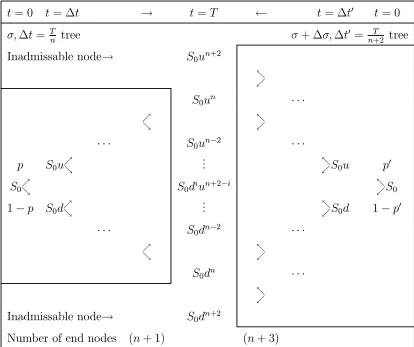
[image:12.595.88.502.108.455.2]Number of end nodes (n+ 1) (n+ 3)
Table 1: Two binomial trees (the larger reversed in time to aid comparison) with
different volatilities and probabilities p, p0, and all final nodes coincident except
two.
in the new tree are again different.4 The detailed tree structures of the modified
binomial method are shown in Table 1, note the two extra nodes (inadmissible for
the first tree), one at both extremes of the final asset price.
Now as volatility is increased one new node is added above and below the exercise
price so that the balance of nodes either side is less likely to change.
Further-more the distance between the exercise threshold and its closest node is likely to
4Probabilities p0 = er∆t0
−d
u−d are smaller than the initial ones p = er∆t
−d
u−d because discount
factorser∆t0 are smaller thaner∆t³∆t0
∆t =
n n+2
´
stay roughly the same (as well as staying the same sign). Thus the potential for
oscillation around the exercise threshold is lessened.
It is worth discussing that, in the spirit of the extended binomial tree method of
Pelsser and Vorst (1994), the modified binomial method and the trinomial method
are both essentially one—tree structures because the trees for two different
volatili-ties share almost all of the same nodes. They share the same stock price nodes so
that each does need separate storage during computation, only the option prices
need separate storage along with the two probabilities. Therefore this method and
the trinomial method will be more computationally efficiently than the other four
methods.
All the above six methods discussed in this paper are not mutually exclusive as
their features can be combined. For example, the idea of BBS method can be
applied to the trinomial or the modified binomial methods. The AMM method
can also be added to the trinomial method to improve accuracy. However we have
considered each method separately in order to evaluate their individual costs and
benefits.
4
Numerical results
In order to investigate the convergence properties of Vega by method, numerical
values were calculated for the initial and perturbed volatility (σ = 40%, ∆σ =
σ³qn+2n −1´) and investigated using differing numbers of total steps in the tree. The same volatility perturbation was used across all methods to ensure a fair
comparison.
methods show dollar errors against the known theoretical value (Black Scholes).
Panels A to F in Figure 2 show the dollar errors for the two volatilities in scatter
graph form for the six methods. Finally, Panels A to F in Figure 3 show the
resulting numerical Vega derived from the perturbation around the initial volatility
for the six methods (again as a function of number of time steps).
Table 2 shows the root mean square errors for each method for n from 20 to 100
and 500 to 1,000 and finally Figure 4 shows this information in graphical form,
scattering the (log) r.m.s. errors against the (log) computational time in seconds.
4.1
Binomial method
It is known in the literature that numerical values oscillate around the true limiting
values (the benchmark n → ∞ Black-Scholes value in this case) as n increases.
The results here show that this oscillatory convergence is a problem for estimation
of Vega as well as other of the so called Greeks (partial derivative hedge ratios).
Firstly, Panel A of Figure 1 reaffirms the result, that neighbouring values (in n
the number of steps) have pricing errors which are negatively serially correlated.
Panel A of Figure 2 shows that although these errors are correlated, they are not
perfectly correlated and that there is considerable dispersion around the 45 degree
line.
Consequently when (for a fixed level of time steps n) numerical differentiation is
employed via a perturbation ∆σ in σ (Equation 1), the resulting Vega oscillates
around its Black Scholes theoretical value (Panel A of Figure 3). Convergence is
slow in n and the envelope for Vega is roughly a tenth of its level (for small n).
Thus as noted by many other authors for option Deltas, the binomial method is
4.2
AMM method
The Adaptive Mesh Model reduces the pricing error by adding more nodes to the
tree in the region near exercise. As can be seen from Panel B of Figure 1, the
resulting prices are indeed considerably more accurate than the Binomial method.
For both option estimates (the unpeturbed and volatility peturbed) the error
en-velope is considerable smaller than in the previous case and more importantly the
errors are no longer so negatively serially correlated (across n).
Furthermore the scatter graph of pricing errors under the AMM (Panel B of Figure
2) is much tighter to the origin, but although it has less dispersion along the 45
degree line, the correlation of these errors is smaller than for the regular Binomial
method because the dispersion in the perpendicular to the 45 degree line has not
been reduced by the AMM method.
Although it does reduce the pricing error, the AMM method inherits and indeed
magnifies the relative dispersion of the pricing errors. Other methods may produce
larger overall errors, but if these errors across two values of σ are more dependent
they will be easier to eliminate.
Thus the numerical Vega estimates in Panel B of Figure 3 (although not as
os-cillatory) still only tracks the true Vega within a large (but converging) envelope.
This is true for this and the Binomial method because although the effect of
dis-cretization can be reduced, its effect on the error structure and correlation cannot
be eliminated.
The next pair of methods behave differently and eliminate this last problem but
4.3
BBS method
The so called Binomial Black Scholes method (BBS) smooths out the option value
function through the addition of the continuous Black Scholes pricing function one
period before maturity. Thus as the number of time steps is varied there are no
final nodes that can oscillate around the payoff condition.
In terms of price accuracy, the BBS performs well (Panel C of Figure 1).
Further-more, the errors while small in magnitude are also highly correlated. However, the
errors decrease at different rates as n increases, therefore the difference in errors
is not expected to be zero. This leads to the situation where Equation 1 is
incon-sistent due to the non zero mean error difference. The best situation for the two
errors is that their best fit line is of unit slope and passes through the origin with
a tight fit. Then both errors are highly dependent and their difference is much
smaller. The scatter graphs in Panel C of Figure 2 contain the 45 degree line for
reference.
As can be seen for Panel C of Figure 2, this is not the case for the BBS method so
the numerical Vega contains error bias. Thus the numerical Vega (in Panel C of
Figure 3) although stable across choice of nis inconsistent for all but the highest
number of step. This is to say that the option price difference for the higher
volatility less the lower is too low compared to the volatility difference itself.
4.4
HZ method
Like the BBS, this method applies smoothing. The D Panels tell a similar story.
Price errors themselves are large and declining almost monotonically withn(Panel
are not consistent. Their regression line is not of unit slope; it is greater than one
so that the error difference again is not zero.
Unlike the previous case, the higher volatility price contains a higher mean error
than the lower case as can be seen in Panel D of Figure 2. As a consequence, the
Vega estimate is overestimated and converges from above but only slowly (Panel
D of Figure 3).
Both of these last two methods that smooth the value function (BBS and HZ) thus
lead to less precise Vega estimates even though they may produce prices that are
in themselves more accurate. This is because of the structure present in the errors.
The next two methods seek to exploit some of the similarity properties of the tree
node structure in each volatility case and therefore produce a smaller overall error.
4.5
Trinomial method
The trinomial tree method performs quite well in Vega estimation. Price errors are
highly correlated and have a bestfit very close to the unit slope, zero intercept line.
Thus the errors cancel out well in the numerical Vega estimation and although
upward biased (the higher volatility option has the higher error) they converge
quite well as nincreases.
These results are somewhat akin to those of the Binomial method since two
bino-mial steps (with recombination) produce a very similar tree to that of a trinobino-mial.
Looking at Panel A of Figure 1, if alternate points as a function of n (say for
even n) were considered the results would be similar to the trinomial tree. Indeed
the (upper) envelopes of the price and Vega curves for the BBS are similar to the
Therefore it may seem as if the results for the Binomial method could have been
substantially improved through the use of even nordinates only, which would be
equivalent to comparing two trinomial trees similar to Ritchken’s method. However
when we tested this method it only seemed to eliminate the oscillatory convergence
in the special case where the initial stock price S equalled the exercise price K.
For other S/K ratios, the Vega still converged in an oscillatory fashion.
Overall as can be seen from Panel E of Figures 1 to 3, the Trinomial method while
containing some bias, works quite well in terms of Vega estimation.
4.6
MB method
Finally the Modified Binomial method (MB) is presented. Because it does not
add more nodes near expiry or attempt to smooth out the value function by an
insertion of a functional form near expiry, the pricing errors are large and suffer
the regular oscillatory convergence problem. For this method to work the volatility
perturbation has to be chosen to depend onnin a particular fashion (withσ = 40%
and σqn+2
n ).
5
Panel F of Figure 1 shows the price of two options . However because of the
positioning of the final nodes, these errors are both highly correlated and nearly
on the unit slope zero intercept line as can be seen from the scatter plot in Panel
F of Figure 2.
As a consequence, the Vega estimates in Panel F of Figure 3, although oscillatory,
have low error, are within a tight envelope and converge quickly. This is in contrast
5This choice of volatility perturbation is required for the MB method to work but has also been
adopted for all other methods to ensure comparability of results. It also has the useful property
to all previous methods. In many applications, this MB method would be highly
suitable for robust, quick and accurate Vega calculation. This is because it uses
only two extra (and uniquely different) nodes so the maximum amount of nodes
are common to both trees.
5
Comparison of RMS errors and times
Table 2 shows root mean squared errors for 243 option prices for each of the six
methods. For all 35 = 243 combinations of parameters drawn from combinations
of K ∈ {35,40,45}, T ∈ {1,4,7} months, σ ∈ {20,30,40}%, r ∈ {3,5,7}%,
q ∈ {2,5,8}% (dividend yield) numerical Vegas were calculated using ∆σ =
σ³qn+2n −1´ for the peturbation.
The errors against the Black Scholes continuous value were squared, averaged and
square rooted to produce an aggregate RMS statistic. This was done repeatedly for
differing numbers of time steps n∈{20,40, ..,100,500,1000} in order to examine
the convergence properties. The time taken for computation is also shown in
minutes, seconds and hundredths of seconds.
Each method almost always yields a lower RMS for increased n (the binomial
method being the most striking exception for lower values of n). Computational
time always increases with nand all methods require a similar magnitude of time
to compute apart from the BBS (which requires normal integrals). However the
AMM and the trinomial method take about twice the time of the binomial, HZ
and MB methods because of their extra tree complexity.
For many values of n and especially for large n, the binomial method and AMM
between the errors for differing volatilities. Surprisingly the BBS method also
performs poorly for lownas well, however its performance improves asnincreases
although this comes with increased computational burden. Although the BBS
price errors are well correlated across the volatility and its perturbed value, their
slope is not unity so that the Vegas calculated using this method contain bias.
The final three methods (Trinomial, HZ and MB) are quite similar in terms of
RMS performance and speed, however (like the AMM method) the Trinomial
cal-culation that contains more nodes and paths takes longer to evaluate than the HZ
and MB methods. The new Modified Binomial method performs quite similarly
to the HZ method but its errors are always lower for comparable computational
times. Furthermore its simple tree design lends it more intuitive appeal. This
is remarkable given the lack of price accuracy inherent in the Modified Binomial
method, however the high price coincidence across volatilities (Figure 1F) and very
high correlation between errors (Figure 2F) means that error cancellation is almost
complete in Vega calculation.
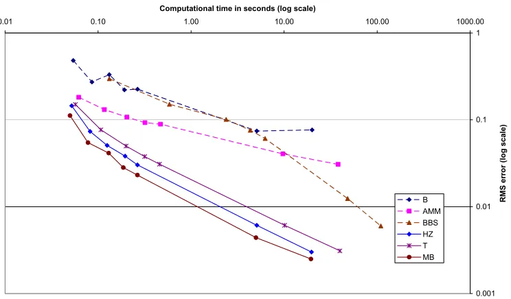
Figure 4 also shows the RMS errors and times from Table 2 in scatter plot form.
The horizontal axis details computational time in seconds, while the vertical details
RMS errors (both in log10 scale). The points on the left of Figure 3 are for n= 20
and move to n = 1,000 on the right. This graphic reiterates the results just
discussed that the Modified Binomial method gives an easy way to achieve quick
and accurate estimates of option Vegas.
6
Conclusion
In conclusion, the model that produces the most accurate option prices may not
erenti-ation. This is because the error in the Vega depends not only on the magnitude
of the errors present in the two price estimates, but critically on their correlation
structure.
Models that produce individually accurate but jointly inaccurate prices such as the
AMM or BBS will not be good for estimating option Vegas (and other Greeks).
Models that are tailored specifically to reduce the discretization error near a
ter-mination boundary however, do much better in terms of Vega estimation.
These models, such as the Modified Binomial (MB) presented here, are the ones
that are also most likely to produce the best Vega results for other option types such
as American and Barrier, where no closed form benchmark formulae are available.
7
References
Amin, K. I., 1991, On the Computation of Continuous Time Option Prices Using
Discrete Approximations, Journal of Financial and Quantitative Analysis, 26,
477-495.
Boyle, P., and S. H. Lau, 1994, Bumping Up Against the Barrier with the Binomial
Model, Journal of Derivatives, 1, 6-14.
Broadie, M., and J. Detemple, 1996, American Option Valuation: New Bounds,
Approximations, and a Comparison of Existing Methods, Review of Financial
Studies, 9, 1211-1250.
Chung, S. L., and M. Shackleton, 2002, The Binomial Black-Scholes Model and
Figlewski, S., and B. Gao, 1999, The Adaptive Mesh Model: a New Approach to
Efficient Option Pricing, Journal of Financial Economics, 53, 313-351.
Heston, S., and G. Zhou, 2000, On the Rate of Convergence of Discrete-Time
Contingent Claims, Mathematical Finance, 10(1), 53-75.
Hull, J. 2000, Options, Futures and other Derivatives, Prentice Hall, Fourth
Edi-tion.
Omberg, E., 1988, Efficient Discrete Time Jump Process Models in Option Pricing,
Journal of Financial Quantitative Analysis, 23, 161-174.
Pelsser, A., and T. Vorst, 1994, The Binomial Model and the Greeks, Journal of
Derivatives, 45-49.
Ritchken, P., 1995, On Pricing Barrier Options, Journal of Derivatives, 19-27.
Tian, Y. 1999, A Flexible Binomial Option Pricing Model, The Journal of Futures
Markets, 19, 817-843.
Widdicks, M., A. D. Andricopoulos, D. P. Newton, and P. W. Duck, 2002, On
the Enhanced Convergence of Standard Lattice Methods for Option Pricing, The
Table 2: RMS (root-mean-squared) errors of six Vega estimates
Number of steps 20 40 60 80 100 500 1000
Binomial 0.4817 (0:00.054) 0.2727 (0:00.086) 0.3313 (0:00.132) 0.2211 (0:00.192) 0.2254 (0:00.266) 0.0743 (0:05.083) 0.0766 (0:19.974) AMM 0.1818 (0:00.062) 0.1311 (0:00.117) 0.1075 (0:00.204) 0.0927 (0:00.320) 0.0890 (0:00.469) 0.0406 (0:09.696) 0.0307 (0:38.093) BBS 0.2971
(0:00.132) 0.1511 (0:00.584) 0.1010 (0:02.383) 0.0759 (0:04.326) 0.0609 (0:06.243) 0.0124 (0:48.092) 0.0060 (1:49.478) HZ 0.1452
(0:00.052) 0.0736 (0:00.082) 0.0507 (0:00.125) 0.0382 (0:00.195) 0.0303 (0:00.265) 0.0061 (0:05.085) 0.0030 (0:19.730) Trinomial 0.1502 (0:00.057 0.0767 (0:00.107) 0.0498 (0:00.200) 0.0378 (0:00.317) 0.0309 (0:00.458) 0.0061 (0:10.127) 0.0031 (0:39.822) Modified binomial 0.1118 (0:00.050) 0.0546 (0:00.078) 0.0414 (0:00.130) 0.0282 (0:00.187) 0.0231 (0:00.265) 0.0044 (0:04.984) 0.0025 (0:19.460) RMS=
∑
= 243 1 2 243 1 i ie defines the root-mean-squared errors for European puts where the
error ei =(Vi*−Vi) depends on Vi is the accurate (closed form) European Vega, Vi*
the estimated Vega using σ and σ((n+2)/n)0.5. There are 243 parameter sets used:
S=40, and combinations of K=35, 40, 45, σ=0.2, 0.3, 0.4, T=1, 4, 7 months, r=3, 5, 7 %, and q=2, 5, 8%. The CPU time (in minutes, seconds, hundred of seconds) required to value all 243 options is also given.
Figure 4: RMS error against computational time for six Vega estimation methods
0.001 0.01 0.1 1
0.01 0.10 1.00 10.00 100.00 1000.00
Computational time in seconds (log scale)
[image:26.595.104.476.483.701.2]