Application of Geophysical Methods for Geotechnical Parameters Determination at New Borg El Arab Industrial City, Egypt

http://dx.doi.org/10.4236/cus.2014.21003

How to cite this paper: Basheer, A. A., et al. (2014). Application of Geophysical Methods for Geotechnical Parameters De-termination at New Borg El-Arab Industrial City, Egypt. Current Urban Studies, 2, 20-36.

http://dx.doi.org/10.4236/cus.2014.21003

Application of Geophysical Methods for

Geotechnical Parameters Determination at

New Borg El-Arab Industrial City, Egypt

Alhussein A. Basheer*, Abdelnasser M. Abdelmotaal, Hany S. Mesbah, Khamis K. Mansour Geomagnetic and Geoelectric Department, National Research Institute of Astronomy and Geophysics, Helwan, Cairo, Egypt

Email:*[email protected]

Received 25 January 2014; revised 10 February 2014; accepted 1 March 2014

Copyright © 2014 by authors and Scientific Research Publishing Inc.

This work is licensed under the Creative Commons Attribution International License (CC BY).

http://creativecommons.org/licenses/by/4.0/

Abstract

Due to a rapid increase in the population during the last few decades, the banks of the Nile River and its delta have reached maximum capacity. As a consequence of this increase, the Egyptian Government has constructed a number of new urban areas and industrial cities outside the Nile Delta. New Borg El-Arab City is one of these new industrial cities. This city is located around 60 km southwest of Alexandria City. This industrial city is proposed to include an airport, a number of factories, worker settlements and heavy truck roads. Therefore, a detailed study of site charac- terization should be performed before construction being in order to. The main target of this study is to determine the dynamic characteristics and geotechnical parameters at the proposed site using seismic refraction and electrical resistively techniques. Analysis and interpretation of the obtained results reveal that the subsurface consists of three layers with a gentle general slope toward the Mediterranean Sea. The classification of rock material for engineering purposes re- veals that the study area is divided into three zones.

Keywords

ERT; SSR; Geotechnical Properties; New Borg El-Arab Industrial City; Egypt

1. Introduction

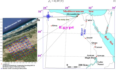
New Borg El-Arab industrial zone is one of the new industrial cities in Egypt. It lies between latitudes 30.75043221 and 31.04684093 N and longitudes 29.44052705 and 29.6723497 E, covering an area of about 90

km2 (Figure 1). This new industrial city is an urbanization project that is relatively large-scale regional devel- opment project and it will be good if the determination the dynamic characteristics and geotechnical parameters being incorporates in the planning stage. So, the main target of the present study is investigating the shallow subsurface structure conditions, the dynamic characteristics and geotechnical parameters of subsurface rocks using shallow seismic refraction profiling and electrical resistivity tomography surveys. The output of this study is very important for solving problems, which associated with the construction of various civil engineering pur- poses, land use-planning and earthquakes resistant structure design. The integrated interpretation of these tech- niques classifies the subsurface succession into three layers.

2. Geological Setting

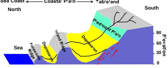
According to (El Shaazly, 1964), the geological setting of the study area is similar environment consisting of Quaternary deposits (scattered), Oligocene (Sand), Beniolitic Clay, and Middle Miocene as Limestone (from top to bottom), Figure 2. The geomorphological units west of Alexandria showed by (Abd El Mawla, 2010) as in Figure 3.

3. Methodology

In the present study two from the advanced technuqes have been applied; electrical resistivity tomography and shallow seismic refraction. Electrical resistivity tomography is a geophysical technique for imaging and map- ping the vertical and horizontal sub-surface structures from electrical resistivity measurements made at the sur- face. The shallow seismic refraction technique is considered as one of the most effective geophysical method, which can be applied in the field of engineering seismology i.e. tunnels, dam sites, landslides, quarries, roads, reclemaited lands, caves and cavities.

3.1. Electrical Resistivity Tomography

In the ERT method the distribution of the electrical resistivity of the subsoil is obtained by injecting electrical current (by the current electrodes) into the ground and measuring the potential difference (by the potential elec- trodes) at two determined points of the surface. The method is based on the application of Ohm’s law:

(

)

a k V I

ρ = ∆ (1)

Figure 2. Geological map of the study area, west of Bourg El-Arab(after GNBCC, 2012).

Figure 3.Geomorphological units west of Alexandria (after Abd Elmawla, 2010).

where ρa is the apparent resistivity (Parasnis, 1997), k is a geometric constant that depends only on the recipro-cal positions of the current and potential electrodes; ΔV is the measured potential difference, and I is the inten-sity of the injected current. The apparent resistivity values depend on the true resistivity distribution.

The true resistivity distribution in the investigated medium can be estimated by an inversion procedure based on the minimization of a suitable function. This function is generally the sum of the squared difference between measured and calculated apparent resistivities. The investigated medium is discredited in a 2D (or 3D) grid of cells, where each cell is assigned an initial resistivity value. A finite-difference (Dey & Morrison, 1979a, b) or finite-element (Silvester & Ferrari, 1990) procedure computes the predicted apparent resistivity at the surface. The solution to the problem, as is well known, is not unique. For the same measured data set, there is wide range of models that can give rise to the same calculated apparent resistivity values. To narrow down the range of pos-sible models, normally some assumptions are made concerning the nature of the subsurface (i.e. geology of the subsurface, whether the subsurface bodies are expected to have gradational or sharp boundaries) that can be in-corporated into the inversion subroutine. The current method of solution minimizes the difference between measured and calculated apparent resistivities using the smoothness-constrained inversion formulation, which

Sea

90

60

30

0

constrains the change in the model resistivity values to become smooth (Loke & Barker, 1996; Loke, 2001). The “smoothness-constrained robust inversion” method (Loke, 2001) has proved to be much more useful when the subsurface bodies have sharp boundaries (Loke, 2001).

3.1.1. ERT Data Acquisition

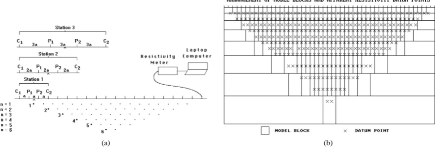
The ERT measurements are carried out along 56 profiles oriented approximately N-S (Figure 1). For this type of data set, a series of 2D inversions is usually first carried out. The 3D inversion is then used on a combined data set with the data from all the survey lines. Apparent resistivity data were collected using the Syscal R2D in- struments in multi-electrode configuration. The distance between profiles was 2 km and a total of 24 electrodes spaced at 5-m intervals are employed. Data are collected using the pole-pole array. The pole-pole array was cho- sen because, as is well known, it is very sensitive to horizontal changes in resistivity, and is therefore suitable for mapping vertical and horizontal structures (Loke, 2001). Figure 4 shows the principle of ERT technique.

3.1.2. ERT Data Processing and Interpretation

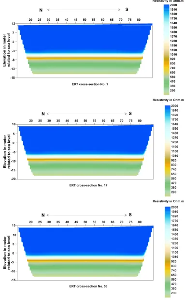
The least-square inversion by Jacobian matrix calculation was used in order to obtain an image of the true resis- tivity distribution as a function of depth. The least-square inversion method (Loke, 2001) minimizes the absolute changes (l1-norm) in the model resistivity values (Loke, 2001). All pole-pole inverted resistivity sections pro- duced low RMS errors (<13%). The Res2dinv software (Loke, 2001) is used to invert all 2D and 3D data sets. Figure 5shows an example for inverted resistivity section with tomography data along profiles “1, 17, and 56”.

As the measured sections are straightforward to combine all 2D images and produce resistivity slices for dif- ferent depths. The Res3dinv resistivity inversion software (Loke, 2001) is used to automatically invert the ap- parent resistivity acquired data and to yield a three-dimensional resistivity model. The slicer-cubic software

(Samuil, 2008) is used to automatically draw output interpreted resistivity data from Res3dinv software to ac- quiesce a three-dimensional resistivity model (Figure 6). From this figure it can be concluded that, the topmost layer presents a larger area with high resistivity variations over short distances (about 2100 Ωm to 1500 Ωm). In comparison, second layer, lying at a depth ranging from 13.35 to 16.75 m, shows more gradual lateral variations in the model resistivity values, this layer presents moderately resistivity values (ranging from 1500 Ωm to 600 Ωm). Third layer lying at a depth varies between 22.25 and 24.60 m. The resistivity values of it are clearly visi- ble, ranging from about 600 Ωm to about 200 Ωm.

3.2. Shallow Seismic Refraction Tomography (SSRT)

Many researchers have used seismic refraction technique to determine the characteristics of the sites, and the necessary parameters for constructions (e.g. (Dutta, 1984), (Marzouk, 1995), (Mohamed, 1993), (El-Behiry, 1994), (Hatherly, 1986), (Sjogren & Sandberg, 1979) and (Abdelmotaal, 2010)).

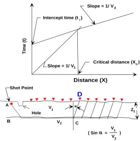
Seismic exploration involves generation of seismic waves and recording the arrival times of these waves from the source to the series of geophones (Figure 7). Seismic refraction is used to evaluate the necessary parameters

(a) (b)

Figure 6. Three-dimensional resistivity model of the study area.

Figure 7. Velocity estimation using the slope method calculation with shot point and geophones array in field.

for constructions, or to solve the problems related to the geological nature of sub-surfaces, mining works, and the environmental conditions overcame in the site (Stumpel et al., 1984).

In the shallow seismic refraction method, the seismic waves, created by artificial sources such as an auto-hammer viberator, propagate through the medium and are refracted at interfaces, where the seismic veloc-ity or densveloc-ity changes. Geophones laid on a single line record the waves returning to the surface after travelling

D

T

im

e

(

t)

Intercept time (t )

Slope = 1/ V

Slope = 1/ V₁ Critical distance (X )

2

i

c

Distance (X)

Shot Point

A

B

V

V _C

1

2

1

Z

( Sin = ) V₁

different distances through the ground. By measuring the travel time between the break and the recording of a seismic signal, the seismic velocity in the subsurface and the depth of the interfaces may be inferred. Figure 7 schematic diagram shows the principle of the shallow seismic refraction.

Conventional analysis of seismic refraction data sets makes simplified assumptions about the velocity struc-ture that conflict with observed heterogeneity, lateral discontinuities, and gradients (Parasnis, 1997). Refraction tomography is designed to resolve velocity gradients and lateral velocity changes, enabling it to be applied in settings where traditional techniques fail.

The method used in this paper utilizes non-linear travel time tomography consisting of ray tracing for forward modeling and simultaneous iterative reconstruction technique (SIRT) for inversion. In this method, the velocity model is represented by quadrangle cells (Figure 8). The width of each cell is chosen as the receiver interval. First-arrival travel times and ray paths are calculated by the ray tracing method based on Huygen’s principle

(Parasnis, 1997). A ray is expressed as a line connecting the nodes arranged on the cell and the travel time be-tween a source and a receiver is defined as the fasted travel time of all ray paths (Figure 8). A model is updated by the SIRT (for more information see (Morey & Schuster, 1999), (Nemeth et al., 1997).

3.2.1. SSRT Data Acquistion

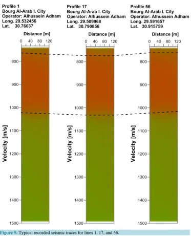
The target to be executed was the determination of dynamic properties of soil and foundation rocks by using seismic refraction method and this implied firstly to throw light upon the end product of seismic refraction tech-nique that was used in this study. Shallow seismic refraction techtech-nique was applied in the present study to de-termine the subsurface layering and its dynamic characteristics at the study area. The seismic refraction data have been acquired along 56 shallow seismic refraction profiles spread over the same area proposed for the R2D resistivity imaging survey (Figure 1). The survey has been accomplished using 24 channels signal enhancement seismograph “GEOMETRICS SMARTSEIS” along 120 m length profiles. Three shots are selected on the seis-mic line for measuring perpendicular and surface waves: two near shots at the edges of the line, and one shot at the middle of the line. In the surface P and SH wave velocities have been measured. The hammer connects to sensor to provide the time break to the seismograph. The power of the hammer helps to avoid loosing of waves strength that may be caused by Blind layer in some condition. The low pass filter in the recording system has 7 - 10 MHz as frequency response, which is suitable for the recording condition, positioned before the ana-log-digital conversion circuit. Data were stacked at least three times for each source. Figure 9 shows the meas-ured raw data (typical recorded seismic traces) of profiles number 1, 17, and 56 as examples.

3.2.2. SSRT Data Processing and Interpretation

For interpretation of refraction data an initial depth model is obtained using Gardner’s method (Gardner, 1939). To perform the processing and interpretation of the seismic refraction tomography data in the current study, (SIPEEDIT (V. 3) 2002) software developed by OYOO Company is used. Therefore, an initial velocity model is estimated. In this case, the initial velocity model is represented by the results obtained from the simple interpre-tation of refraction data (such as the model shown in Figure 9). The model is represented by 1-1 m cells. Re-fraction rays are traced through this model to give calculated travel times. A misfit function, consisting of the squared difference between the observed and computed travel times, is calculated. The model is adjusted until the misfit is minimized. The iterations are stopped when the RMS travel time residual (difference between

Figure 9. Typical recorded seismic traces for lines 1, 17, and 56.

the calculated travel times for the initial model and the observed ones) is less than the average travel time pick error.

3.2.3. SSRT Velocity

Vs velocity between 669 to 781 m/s, those correspond to sandy marl layer strongly cemented with depth vary from 25 and 26 m where the ERT profile shows the moderate resistivity values. The third layer is characterized by the highest seismic velocities (Vp and Vs), corresponds to the area about where the ERT profile shows the lowest resistivity values. The grey zone presents the no-ray area.

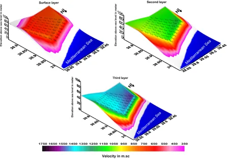
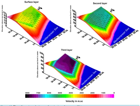
The increase of seismic wave velocity could be due to a more compact soil (calcareous sands weakly ce-mented). According to the variation in Vp and Vs velocities are detected, four cross-sections, over the study area, have been drawn to show the distribution of these layers in the four sides (Figures 10-13). Three dimension maps of the distribution of Vp and Vs velocities for the three layers over the study area are shown inFigures 14 and 15.

Figure 10. Depth cross-section along profiles (1, 9, 17, 25, 33, 41, and 49).

Figure 11. Depth cross-section along profiles (8, 16, 24, 32, 40, 48, and 56).

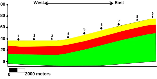
Figure 12. Depth cross-section along profiles (1, 2, 3, 4, 5, 6, 7, 8, and 9). 2000 meters South North 30 20 10 0 40 50 9 17 25 33 41 49 Sea 2000 meters South North 60 40 20 0 80 100 16 24 32 40 48 56 Sea 100 80 60 40 20 5 6

0 2000 meters

Figure 13. Depth cross-section along profiles (49, 50, 51, 52, 53, 54, 55, and 56).

Figure 14. Three-dimension velocity map for seismic perpendicular waves.

4. Geotechnical Paramters

4.1. Density Gradient (Di)

There is a direct relation between the material competence and the value of the density gradient and the com-pression velocity (Vp). “The compaction” can be defined as “name of the physical mechanism that converts sediments from their initial state to a progressively denser state under the influence of their own weight or of tectonic movements” (Cordier, 1985). The density gradient (Di) relates to how much consolidation or settlement will take place. Many relations can express it “according to Stumpel et al. (Stumpel et al., 1984)”

(

)

Di= Vp2−4 3 Vs2 −1 (2) 75

60

45

30

15

49 50 51 52

53

54

55

56

West East

Figure 15.Three-dimension velocity map for seismic surface waves (Vs).

The distribution of the density gradient in the subsoil layers has been shown in Figure 16. Generally over the three layers, the relatively low values are observed in the southeastern part of the study area, which indicates the relatively moderate competent materials. The middle values are occupied in the middle part that may be due to difference in sorted materials. While the high values are observed in the northwestern part of the study area, they reflect the fairly moderate competent materials in this part of the study area. Table 1 shows the distribution of the density gradient.

4.2. Standard Penetration Test (SPT) [N-Value]

The Standard Penetration Test (SPT) is geotechnically known as “the resistance to penetration by normalized cylindrical bars under standard load”. N-value is geophysically evaluated using Imai’s (Imai, 1976; Stumpelet al., 1984), which is given by the formula:

Vs=89.9N0.341 (3)

Table 2 shows the distribution of N-Value. In general for the three layers of the study area, Figure 17 shows the comparatively low values that are experimented in the southeastern part of the study area, which point to-ward the relatively moderate competent materials. The middle values are inhabited in the middle part that may be suitable to difference in sorted materials. Whereas the high values are observed in the northwestern part of the study area, they reflect the fairly moderate competent materials in this part of the study area.

4.3. Kinetic Bulk Modulus (K)

Figure 16. Three-dimension map of density over the study area.

Table 1. The distribution of the density gradient of the study area.

Subsoil layers Density gradient Surface layer 2.67 × 10−6 to 2.97 ×10−6 Second layer 1.36 ×10−6 to 1.65 ×10−6 Third layer 6.72 ×10−7 to 7.67 ×10−7

Table 2. The distribution of (N-Value) over the study area.

Subsoil layers Standard penetration test (N-Value)

Surface layer 78 to 89

Second layer 172 to 269

Third layer 404 to 567

( )

K= ⋅ρ _Vp2− 3 4 Vs2_ (4)

where ρ is the density.

Table 3 shows the division of Bulk modulus. Over the three subsoil layers, the minimums values of Bulk modulus are observed in the southeastern part of the study area. These values increase to be moderate ones in the center part, while the maximum values are observed in the western and the northwestern corners of the study area (Figure 18).

4.4. Ultimate Bearing Capacity (Qult)

Figure 17. Three-dimension map of Standard penetration Test [N-Value] over the study area.

Table 3. The distribution of Kinetic Bulk modulus (K) over the study area.

Subsoil layers Kinetic Bulk modulus Surface layer 528 to 648 Dyn/Cm Second layer 1803 to 3387 Dyn/Cm

Third layer 6016 to 9681 Dyn/Cm

quefaction”. This capacity is controlled by shear strength factor. The ultimate bearing capacity for cohessionless soils can be calculated by using the standard penetration test (SPT) from Parry’s formula (Parry, 1977) as:

Qult=30N (5)

where “N value” is the resistance to penetration by normalized cylindrical bars under standard load.

Figure 19 shows the overview of the three layers in the study area. The minimums values of ultimate bearing capacity are observed in the southeastern part of the study area. These values increase to be moderate ones in the center part, while the maximum values are observed in the north and the northwestern corners of the study area. Table 4 reveals the distribution of the ultimate bearing capacity (Qult) in the subsoil layers of the study area.

4.5. Allowable Bearing Capacity (Qa)

The allowable bearing capacity is the maximum load to be considerable to avoid shear failure or sand liquefac-tion. It can be termed as allowable bearing pressure too, the foundation materials are affected by both strength and deformation characteristics.

The allowable bearing capacity can be calculated by dividing the ultimate bearing capacity value (Qult) by suitable factor of safety (Abd Elrahman, 1989) as:

Figure 18. The allotment of Kinetic Bulk Modulus (K) in the study area.

The safety factor (F) equals 2 when the soil is cohessionless and equals 3 when the soil is a cohesive material. Table 5 reveals the distribution of the allowable bearing capacity (Qa) in the subsoil layers of the study area. The minimum values of allowable bearing capacity are observed in the southeastern part of the study area. These values increase to be moderate ones in the center part, while the maximum values are observed in the north and the northwestern corners of the study area (Figure 20).

4.6. Rock Material Calssification

This study suggests the classification of foundation rock materials in the study area for engineering purposes based on all the calculated moduli and parameters (Figure 21). This study is divided (the selected study area only) into:

1-Zone (A): (competent material zone):

This zone covers the northwestern corner and the small strip in the middle quarter of the study area. Good competent materials characterize this zone suggesting suitability for any engineering purposes.

2-Zone (B): (Moderated competent material zone):

This zone covers the middle quarter with small strip in the southwestern part of the study area. This zone suggests suitability for moderately and low-load engineering purposes.

3-Zone (C): (non-competent material zone):

This zone covers the eastern part of the study area with some extent in the north. This zone consists of less competent materials not suitable for limited construction purposes. This zone is suggesting non-suitability for any engineering purposes that must be kept away from any constructions or loadness and watery activities.

5. Discussions and Conclusions

Figure 19. Three-dimension map of the ultimate bearing capacity over the study area.

Table 4. The ultimate bearing capacity (Qult) over the study area.

Subsoil layers The ultimate bearing capacity (Qult) Surface layer 2211 to 2950 K.Pa Second layer 5827 to 7793 K.Pa Third layer 12131 to 1707 K.Pa

Table 5. The allowable bearing capacity (Qa) over the study area.

Subsoil layers The allowable bearing capacity (Qa) Surface layer 1105 to 1475 K.Pa Second layer 2594 to 3915 K.Pa

Third layer 6065 to 8503 K.Pa

and shallow seismic-refraction tomography (SSRT) methods are used. The results highlight the reliability of the integrated data interpretation based on two physical parameters with different resolution and sensibility.

Electrical survey, effectively visualized as iso-resistivity surfaces, classified the area into three layers. Shal-low seismic refraction tomography correlates well with ERT. The integrated interpretation of seismic refraction and resistivity tomography makes it possible to reduce ambiguity. The proposed method of 3D visualization (iso-resistivity and iso-velocity) confirms the interpretation of the 2D standard horizontal sections.

Figure 20. Three-dimension map of the allowable bearing capacity over the study area.

Figure 21. Classification of the foundation rock material quality for engineering purposes according to the geotech-nical characteristics in the study area.

29.46 29.48 29.5 29.52 29.54 29.56 29.58 29.6 29.62 29.64 29.66

30.76 30.78 30.8 30.82 30.84 30.86 30.88 30.9 30.92 30.94 30.96 30.98 31 31.02 31.04

Competent material zone

Moderated competent material zone

Low competent material zone

A

into three zones of foundation rock material related to the engineering purposes.

References

Abd Elmawla, S. H. (2010). National Workshop. Alexandria.

Abdelmotaal, A. M. (2010). Engineering Seismology Studies for Land-Use Planning at the Proposed Tushka New City Site, South Egypt. Ph.D. Thesis, Qena: South Valley University.

Abd Elrahman, M. M. (1989). Evaluation of the Kinetic Moduli of the Surface Materials and Application to Engineering Geologic Maps at Ma’Barrisabah area (Dhamar Province), Northern Yemen. Egyptian Journal of Geology, 33, 228-252.

Cordier, J. P. (1985). Velocities in Refraction Seismology (276 p). Holland: Radial Publisher Company. http://dx.doi.org/10.1007/978-94-017-3641-1

Dey, A., & Morrison, H. F. (1979a). Resistivity Modelling for Arbitrary Shaped Two-Dimensional Structures. Geophysical Prospecting, 27, 1020-1036. http://dx.doi.org/10.1111/j.1365-2478.1979.tb00961.x

Dey, A., & Morrison, H. F. (1979b). Resistivity Modelling for Arbitrarily Shaped Three-Dimensional Shaped Structures.

Geophysics, 44, 753-780. http://dx.doi.org/10.1190/1.1440975

Dutta, N. P. (1984). Seismic Refraction Method to Study the Foundation Rock of a Dam. Journal of Geophysical Prospecing, 32, 1103-1110. http://dx.doi.org/10.1111/j.1365-2478.1984.tb00757.x

El-Behiry, M. G., Hosney, H., Abdelhady, Y., & Mehanee, S. (1994). Seismic Refraction Method to Characterize Engineer-ing Sites. EGS/SEG Proceedings of the 12th Annual Meeting, 85-94.

El Shaazly, M. M. (1964). Geology and Hydrology of Mersa Matrouh Area, Western Mediterranean, Littoral U. A. R. Ph.D. Thesis, Cairo: Cairo University.

Gardner, L. W. (1939). An Areal Plan of Mapping Subsurface Structure by Refraction Shooting. Geophysics, 4, 247-259. http://dx.doi.org/10.1190/1.1440501

GNBCC (2012). Geology of the Nile Basin Countries Conference. Alexandria.

Hatherly, P. J. (1986). Attenuation Measurements on Shallow Seismic Refraction Data. Geophysics, 51, 250-254. http://dx.doi.org/10.1190/1.1442084

Imai, L. (1976). The Functions of Seismic Wave in Ground Material and Its Interpretations. Geophysics, 41, 745-797.

Leucci, G. (2004). I metodi elettromagnetico impulsivo, elettrico e sismico tomografico a rifrazione per la risoluzione di problematiche ambientali: sviluppi metodologici e applicazioni. Ph.D. Thesis.

Loke, M. H., & Barker, R.D. (1996). Rapid Least-Squares Inversion of Apparent Resistivity Pseudosections Using a Quasi-Newton Method. Geophysical Prospecting, 44, 131-152. http://dx.doi.org/10.1111/j.1365-2478.1996.tb00142.x

Loke, M. H. (2001). Electrical Imaging Surveys for Environmental and Engineering Studies. A Practical Guide to 2-D and 3-D Surveys. RES2DINV Manual, IRIS Instruments. www.iris-instruments.com

Marzouk, I. A. (1995). Engineering Seismological Studies for Foundation Rock for El-Giza Province, Bull. of National Re-search Institute of Astronomy and Geophysics (NRIAG). B. Geophysics, 11, 265-295.

Mohamed, A. A. (1993). Seismic Microzoning Study and Its Applications in Egypt. Ph.D. Thesis, Cairo: Ain Shams Univer-sity.

Morey, D., & Schuster, G. T. (1999). Paleoseismicity of the Oquirrh fault, Utah from Shallow Seismic Tomography. Geo-physical Journal International, 138, 25-35. http://dx.doi.org/10.1046/j.1365-246x.1999.00814.x

Nemeth, T., Normark, E., & Qin, F. (1997). Dynamic Smoothing in Cross-Well Traveltime Tomography. Geophysics, 62,

168-176. http://dx.doi.org/10.1190/1.1444115

Parasnis, D. S. (1997). Principles of Applied Geophysics (5th ed.). London: Chapman and Hall.

Parry, R. H. C. (1977). Estimating Bearing Capacity of Sand from SPT Values. JGED, ASCE, 103, 1013-1045.

Samuil, Q. J. (2008). Slicer Cubic 5.0 Manual, Slicer-Cubic Software. Landsub 5, Germany.

SEIPEEDIT (2002). Seismic Interpretation Program Software. New York: OHOO Company. www.Ohoo.com

Sheriff, R. E. (1991). Encyclopedic Dictionary of Exploration Geophysics (3rd ed.). Society of Exploration Geophysicists.

Silvester, P. P. and Ferrari, R. L. (1990). Finite Elements for Electrical Engineers (2nd ed.). Cambridge: Cambridge Univer-sity Press.

Sjogren, B. O., and Sandberg, J. (1979). Seismic Classification of Rock Mass Qualities. Geophysical Prospecting, 27, 409- 442. http://dx.doi.org/10.1111/j.1365-2478.1979.tb00977.x