Variable and Fixed Structure Augmented Interacting Multiple Model Algorithms for Manoeuvring Ship Tracking Based on New Ship Models

Variable- and Fixed-Structure Augmented Interacting

Multiple Model Algorithms for Manoeuvring Ship

Tracking Based on New Ship Models

1

Emil Semerdjiev Ludmila Mihaylova

Bulgarian Academy of Sciences, Central Laboratory for Parallel Processing ‘Acad. G. Bonchev’ Str,. Bl. 25-A, 1113 Sofia, Bulgaria

Phones: (359 2) 979 67 47; (359 2) 979 66 20; Fax: (359 2) 707 273

E-mail: signal@bas.bg, lsm@bas.bg, http://www.bas.bg/test/mmosi/MMSDP.html

The real-world tracking applications meet a number of difficulties caused by the presence of different kinds of uncertainty - unknown or not precisely known system model and random processes’ statistics or due to abrupt changes in the system modes of functioning. These problems are especially complicated in the marine navigation practice, where the commonly used simple models of rectilinear or curvilinear target motions do not match to the highly non-linear dynamics of the manoeuvring ship motion. A solution of these problems is to derive more adequate descriptions of the real ship dynamics and to design adaptive estimation algorithms. After analysis of basic hydrodynamic models, new ship models are derived in the paper. They are implemented in two versions of the recently very popular Interacting Multiple Model (IMM) algorithm. The first one is a standard IMM version using preliminary defined fixed structure (FS) of models. They represent various modes of ship motion, distinguished by their rate of turns. The same rate of turn is additionally adjusted in the proposed new augmented versions of the IMM (AIMM) algorithm by using FS and variable structure (VS) of adaptive models estimating the current change of the system control parameters. The obtained Monte Carlo simulation results show that the VS AIMM algorithm outperforms the FS AIMM and FS IMM algorithms with respect to accuracy and adaptability.

Key words: Interacting Multiple Model (IMM) algorithm, model uncertainty, state and parameter estimation

1. Introduction

Tracking of manoeuvring targets is a problem of a great practical and theoretical interest. The real applications meet a number of difficulties caused by the presence of different kinds of uncertainty due to the unknown or not precisely known system model and random processes’ statistics as well as because of their abrupt changes (Bar-Shalom, 1992, Bar-Shalom and Li, 1993, 1995, Best and Norton, 1997, Lerro, Bar-Shalom, 1993). These problems are especially complicated in the marine navigation practice, where the applied trivial models of rectilinear or curvilinear target motions do not match to the highly non-linear dynamics of the manoeuvring ship motion. A solution of these problems is to derive more adequate descriptions of the real ship dynamics and to design adaptive estimation algorithms. Such a solution is proposed in the paper. New ship models are derived in Section 2 after a brief analysis of the basic hydrodynamic models (Ermolaev, 1981, Ogawa, et al. 1977, Pershitz, 1973, Sobolev, 1976). These models are implemented in new versions of the Interacting Multiple Model (IMM) filter - one of the most cost-effective among the multiple model algorithms used for estimation

of hybrid systems, i.e. systems with both continuous and discrete uncertainties (Bar-Shalom, 1992, Blom and Bar-Shalom, 1988, Li, 1996, Mazor et al., 1998). A brief summary of the basic features of the Bayesian estimation algorithms and especially of the IMM filter is given in Section 3. Section 4 presents the proposed new IMM algorithms. They are based on an appropriate state vector augmentation, which includes the difference between the unknown control parameters and their values fixed in the IMM algorithm. Because of this model augmentation the resulting IMM algorithm is called here augmented (AIMM). Two AIMM algorithm versions are developed and evaluated. The first is a standard IMM version using a preliminary defined fixed set of models and is called a fixed-structure (FS) algorithm (Li, 1999). The models represent various modes of ship motion distinguished

by their control parameter - the ship’s rate of turn. The same rate of turn is additionally adjusted in the proposed new augmented versions of the IMM (AIMM) filter, respectively with fixed structure and variable structure (VS) (variable set of models, estimating adaptively the current change of the system control parameters). The FS and VS AIMM algorithms are given in Section 4, the results from comparative performance evaluation of the considered algorithms - in Section 5. Finally, inferences and recommendations are summarized in Section 6.

2. Model Identification

(

)

dX

dt =K VV U sinψ β− , (1)

(

)

dY

dt =K VV U cosψ β− , (2) d

dt KV ψ _{= ω}

(3)

(

)

d dt

V

L q s

V

L r

U U

ω

β δ ω

= −_ _ + −

2

31 31 31 , (4)

(

)

d dt

V

L q h s r

U

β _{= − β+ β β + δ − ω}

21 1 21 21 , (5)

V =V K_{U V}, (6)

(

)

K V

V

V

V L V

V

U

U

= ( )= = + − − ≤

( ) .

ω _ω

0 1 19 1

2 2 2 1

,

where VU is the uniform (rectilinear) ship velocity. The state vector of the considered model is

[

]

x= X Y, , , , ,ψ ω β V '. It includes the ship coordinates, heading, rate of turn, drift angle and velocity;

δ

is the control rudder angle deviation. The constant hydrodynamic coefficients

q

21,

r

21,

s

21,

h

1,

31

q

,

r

31 and

s

31 depend on the ship geometry, most of all on the ship length L (Voitkounski, 1985).

Equations (3) and (6) illustrate the main feature of the considered dynamics - the non-linear dependence between the ship’s rate of turn and velocity. This is the main difference between the

above model and the other well-known simple models (Bar-Shalom, 1992, Best and Norton, 1997, Lerro, Bar-Shalom, 1993).

Very often (Pershitz, 1973, Voitkunski, 1985) the CT model (1)-(6) is simplified by substituting

the factor

β

with an off-line computed factor:

31 1

31 1 2 0

2 4 r h

s r h q

q δ

β = − + + ,

where:

q

=

q

21

r

31

−

q

31

r

21,

s

=

r

21

s

31

−

r

31

s

21. The system of two first-order differential equations

2 0

2

2 31

pd dt

L

V q

L

V s

U U

ω _{+ ω + δ=}

, (4’)

2p 21 0

d dt

L

VU q s

β _{+ β+ δ =}

, (5’)

where:

p

=

0

.

5

(

q

₂₁∗

+

r

₃₁

)

,

q

*

=

q

∗₂₁

r

₃₁

−

q

₃₁

r

₂₁,

q

₂₁∗

=

q

₂₁

+

h

₁

β

₀. The final CT model (1)-(3), (4’) and

(6) is obtained by setting β ≡0.

The respective discrete-time (DT) model is:

Xk+1 = Xk +TVksinψk, (7)

Yk+1 =Yk +TVkcosψk, (8)

(

)

[

]

ψ ψ τ τ

k k k k k k U

TV

TV T V e k

+1= + Ω +0 5. Ω −Ω , (9)

(

)

Ωk Ωk Ω

TV U

TV

e k e k

+1 = + 1−

τ τ _{, (10)}

(

)

Vk =V KU V =VU + kL

−

1 1 9. Ω2 2 1, (11)

where k=1 2, , ;

T

is the sampling interval, and

τ = −0 5. p+ 0 25. p2−q∗

L , [m

-1

] , ΩU

[

(

)

]

U

V

s sign q

r L = ω = − 31δ+ δ 31β0

31

,









m

rad

.

The full coincidence between the results obtained by the CT model (1)-(6), and these from the derived DT model (7)-(11) is demonstrated in (Semerdjiev et al., 1998). That is why the DT model (7)-(11) is used for true data generation in the further simulations.

The final DT model, suitable for implementation in a Kalman filter, is received on the basis of the assumptions (Semerdjiev et al., 1998, Semerdjiev and Mihaylova, 1998):

• The observed ship manoeuvres with constant rate of turn:

Ωk+1 =Ωk (i.e.

τ

≡0).

• The domain of unknown control parameters Ω_k may be “covered” by a set of three control

parameters corresponding to the three basic kinds of ship motions: uniform motion (ΩU), left and

right turns (ΩL and ΩR):

[

] [

]

Ω Ω Ω Ω= U, R, L = , ,U U−

' '

where U denotes a preset constant rate of turn. The vector Ω covers all ship manoeuvres and system noises in the band

[

−U U,

]

. The particular choice of U is made by taking into account general

considerations from the marine practice and some important international navigation restrictions (Voitkounski, 1985).

• The attempt to introduce a vector of possible ship lengths has been recognised in (Semerdjiev et

al., 1998) as unsuccessful because of the bad distinction of the resulting models. The uncertainty,

concerning the ship geometry has been overcome by introducing a common constant average ship length l=const (Semerdjiev et al., 1998).

So, the final version of the requested ship model takes the following form:

Xi k, +1= Xi k, +TVi k, +1sinψi k, , (12)

Yi k,+1 =Yi k, +TVi k, +1cosψi k, , (13)

ψi k, +1=ψi k, +TVi k, +1Ωi, (14)

Vi k,+1 =K VV i, U k, . (15)

The new state vector is x_{i k,} =

[

X_{i k,} ,Y_{i k,} ,ψ_{i k,} ,V_{U k,}

]

', KV i, = +

(

. il

)

−

1 19Ω2 2 1, and Ω Ω Ω Ω=

[

_U, _R, _L

]

'

[

]

= 0,U U , i,− ' =1 2 3, , .

Another model version, based on the augmented state vector x_{i k}a_, =

[

X_{i k,} ,Y_{i k,} ,ψ_{i k,} ,V_{U k,} ,∆Ω_{i k,}

]

' is

suggested in (Semerdjiev and Mihaylova, 1998):

X_{i k,+}1= X_{i k,} +TV_{i k,+}1sinψ_{i k,} , (16)

Y_{i k,+}1=Y_{i k,} +TV_{i k,+}1cosψ_{i k,} , (17)

(

)

ψi k, +1=ψi k, +TVi k, +1 Ωi +∆Ωi k, , (18)

Vi k,+1 =K VV i, U k, , (19)

∆Ωi k, +1=∆Ωi k, , (20)

where i=1 2 3, , . This model takes into account possible differences ∆Ωi k, between the unknown true

ship rate of turn Ωk and its values Ωi fixed in the IMM algorithm. The influence of ∆Ωi k, on the

It should be noted also that the above models can be used to cover simultaneous heading and velocity manoeuvres. It is only necessary to introduce velocity noise in the rectilinear motion model.

3.

Standard IMM Algorithm

It is known (Bar-Shalom and Li, 1993, 1995) that to estimate the system state within the framework of the Bayesian approach, the computational and storage requirements increase exponentially with time which makes the estimator not implementable in real time. To circumvent this problem, suboptimal estimators with certain hypotheses management, such as pruning and merging, have been used, leading to such algorithms as generalized pseudo-Bayesian (GPB) algorithms of first order (GPB1), of second order (GPB2), and in general, of order r (GPB r ). It has been shown in (Li, 1996, Bar-Shalom and Li, 1993, 1995) that the IMM algorithm is one of the most cost-effective schemes for estimation of hybrid systems. It yields the performance of GPB2 with the lower requirements of GPB1.

The IMM algorithm is a recursive one (Blom and Bar-Shalom, 1988, Bar-Shalom and Li, 1993, 1995, Li, 1996). Each cycle of the algorithm consists of four major steps: interaction (mixing), filtering, mode update and combination. In each cycle, the initial condition for the filter matched to a certain mode is obtained by interacting (mixing) the state estimates of all filters at previous time under the assumption that this particular mode is in effect at the current time. This is followed by filtering (prediction and update) step, performed in parallel for each mode. Then the combination (weighted sum) of the updated state estimates from all filters yields the state estimate.

The standard IMM filter is used here to develop its versions, suitable for ship tracking, taking into account the ship models particularities.

4. Augmented IMM Algorithms for Tracking of Manoeuvring Ships

4.1. Fixed-Structure Augmented IMM Algorithm for Ship Tracking

(

)

( )

xk = f xk−1,Ωk−1 +g Ωk−1 vk−1, (21)

( )

zk =h xk k +wk, (22)

where the state vector xk nx

∈ℜ is estimated based on the measurement vector zk nz

∈ℜ in the

presence of unknown true control parameter Ω Ω

k n

∈ℜ . The mutually independent additive system

and measurement noises vk n_v

∈ℜ and wk n_z

∈ℜ are white and Gaussian: νk ~ N

(

0,Qk

)

,

(

)

wk ~ N 0,Rk . Functions

f

,

g

and

h

are known and remain unchanged during the estimation

procedure.

To estimate the difference ∆Ωi k, between the current true control parameter Ωk and its value Ωi

fixed in the

i

-th IMM model, the system state model is augmented by the next equation:

∆ Ωi k, =∆ Ωi k,−1, (23)

where

∆Ωi k, =Ωk −Ωi. (24)

The state and system noise vectors of the

i

-th augmented model ( i=1,N) can be written in the form:

[

]

x_{i k}a x_{i k i k} nx n

, , '

, ' '

= _∆Ω ∈ℜ + Ω_,ν

[

ν ν

]

ν

i k a

i k

n n

i k

, ,

' ' '

,

= _Ω ∈ℜ + Ω_.

In general, the new augmented model is nonlinear:

(

)

(

)

xi k f x g v

a a i k a

i i k a

i i k i k a

, = , −1,Ω +∆Ω, −1 + Ω +∆Ω,−1 , −1, (25)

(

)

zk h x w

a i k a

i i k k

= , ,Ω +∆Ω, + . (26)

Functions fa(. ), ga(. ) and ha(. ) are known and remain unchanged during the estimation procedure. The equations of the corresponding Extended Kalman Filter (EKF) are derived by linearization of models (25) and (26). Functions f a

(

x_{i k, −1},Ω_i +∆Ω_{i k, −1}

)

and ga

(

x_{i k,−1},Ω_i+∆Ω_{i k, −1}

)

are expanded in

Taylor series up to first-order terms around the filtered estimate

, /

x_{i k}a ₋1_k−1; the function

(

)

ha x_{i k,} ,Ω_i+∆Ω_{i k,} is expanded up to first-order terms around the predicted estimate

, /

x_{i k k}a ₋₁

, / , / , ,

xi k k x K

a

i k k a

i k a

i k

= ₋1+ γ , (27)

(

)

,

, / , / , /

xi k k f x

a a

i k k a

i i k k

−1= −1 −1 Ω +∆Ω −1 −1 , (28)

(

)

γi k k a

i k k a

i i k k

z h x

, , / , /

,

= − ₋1 Ω +∆Ω ₋1 , (29)

(

)

P_{i k k}a _if_{x k}a P_{i k}a _k f_{x k}a Q_{i k}a

i i

, / , , / ,

'

,

−1 =φ −1 −1 −1 −1 + −1, (29)

( )

S_{i k} h_{x k}a P_{i k k}a h_{x k}a R_k

i i

, , , / ,

'

= ₋1 + , (30)

( )

K_{i k}a P_{i k k}a h_{x k}a S_{i k}

i , , / , ' , = ₋ − 1 1

, (31)

( )

P_{i k k}, /a P_{i k k}, /a K_{i k}a, S_{i k}, K_{i k}a, '

= ₋1− , (32)

where Ki k a

, is the filter gain matrix, Pi k k a

, / and Qi k a

, are the estimation error covariance and system

noise covariance matrices, γ_{i k,} and S_{i k,} are the filter innovation and its covariance matrix, the system

and the measurement Jacobian are fx k a

i, −1 = ∂f

(

x

)

∂x

a i k k a

i i k k i k k a

,

, −1/ −1 Ω +∆Ω, −1/ −1 , −1/ −1 and hx k a

i, =

(

)

∂ha x_{i k k}a ∂x_{i k k}a

, / −1 , / −1; φi≥1 is the EKF fudge factor. The restrictions

[

]

Ω ∆Ωi + i k− k− ∈Ωi Ωi

,

, 1/ 1 ,min ,max are imposed to provide minimal models separation.

After the expansion of the ship models (12)-(15) and (16)-(20) in Taylor time-series, three IMM algorithm versions are derived. The IMM algorithm based on model (12)-(15) is further denoted as FS IMM, while the proposed AIMM algorithm based on model (16)-(20) is denoted as FS AIMM.

4.2 Variable-Structure Augmented IMM Algorithm for Ship Tracking

The FS AIMM algorithm can be transformed into a new VS AIMM algorithm by substituting the constant vector of deterministic parameters Ωi with the random vector of control parameters Ωi k, . At

the beginning of each EKF (before the state prediction step) in the IMM algorithm, the last filtered displacement ∆Ω

, /

i k−1 k−1 corrects the old vector of control parameters Ωi k, −1:

Ωi k, Ωi k, ∆Ωi k, /k

= ₋1+ ₋1 ₋1 (Ωi,0 =Ωi), (33)

[

]

Ωi k, ∈Ωi,min,Ωi,max , for all

i

.

After the above operation, the model displacement ∆Ω

, /

i k−1k−1 is set to zero:

∆Ω

, /

i k−1k−1 =0. (34)

Otherwise, it will be taken into account twice in the EKF equations.

Finally, it should be noted, that the proposed here VS AIMM algorithm is general and does not depend on the implemented system and measurement models. It is an adaptive VS IMM algorithm using minimal number of models, self-adjusting their location in continuous parameter domain.

4.3. AIMM Algorithms Implementation

Considering the AIMM algorithms implementation in sea track-while-scan radars, the particular features of these sensors are taken into account by using the next measurement equation:

zk =Hxk +wk,

where H is the measurement matrix,

   

  =

0 0 1 0

0 0 0 1

H ,

and

w

k is a white Gaussian measurement noise with covariance matrix Rk. The polar measurements

“range-bearing” zk =

[

rk, k

]

'

β , are transformed, for convenience, in Cartesian ones:

Xk =rksinβk, Yk =rkcosβk.

The measurement vector acquires the new form zk =

[

Xk,Yk

]

'

. Respectively, the covariance matrix of

the measurement errors becomes (Farina, 1986):

(

)

(

)

R r r

r r

i k

r k k k r k k k

r k k k r k k k

,

sin cos sin cos

sin cos cos sin

= + −

− +



  



  

σ β σ β σ σ β β

σ σ β β σ β σ β

β β

β β

2 2 2 2 2 2 2 2

2 2 2 2 2 2 2 2 ,

where σ_r and σ_β are respectively the range and bearing standard deviations.

f

TK V TK

TK V TK

TK

K

x k

V i U k k i k k V i i k k V i U k k i k k V i i k k

V i i V i i, , , / , / , , / , , / , / , , / , , cos sin sin cos = −               1 0 0 1

0 0 1

0 0 0

ψ ψ

ψ ψ

Ω ;

the respective one based on model (16)-(20) is:

(

)

f

TK V TK

TK V TK

TK TK V

K

x k e

V i U k k i k k V i i k k V i U k k i k k V i i k k

V i i i k k V i U k k V i i, , , / , / , , / , , / , / , , / , , / , , / , cos sin sin cos = − +                

1 0 0

0 1 0

0 0 1

0 0 0 0

0 0 0 0 1

ψ ψ

ψ ψ

Ω ∆Ω .

A hard logic is introduced in all IMM algorithms to avoid an undesired combination of the

estimates

, /

VU k k,

, /

VL k k and

, /

VR k k (Semerdjiev et al., 1998):

, / , / ,

Vi k k =VU k k ( i=2 3, );

, .

/ , / ,

Vk k =VU k k if µU k >0 5,

where

µ

_i,k is the probability of the event: “the

i

-th model is topical at time k”,

/

V_{k k} is the overall

(final) estimate of the ship velocity.

5. Performance Evaluation

5.1 Measures of performance

The performance of the three IMM algorithms is compared by Monte Carlo simulations. The mean error (ME) and the root mean-square error (RMSE) of each state component have been chosen as

measures of performance (Bar-Shalom and Li, 1993). The ME and the RMSE of both estimated coordinates have been respectively combined. Results from 100 independent runs, each one lasting 200 scans (600s, T=3 s) are given.

The simulation parameters of the true model (7)-(11) are standard (Voitkounski, 1985, Semerdjiev

et

al., 1998): q₂₁=0.331, r₂₁ =-0.629, s₂₁=-0.104, h₁ =3.5,q₃₁=-4.64, r₃₁ =3.88, s₃₁ =-1.019,

L=99m, δmin=3 o

, δmax =30

. The chosen initial conditions are: X₀ =Y₀=10000m, ψ0 =45

,

[image:11.595.84.278.568.739.2]

It is assumed that initially the ship moves rectilinearly. The true ship trajectory is presented in Fig.1. The applied pulse-wise rudder angle control law is:

[

]

[

]

δ = δ ∈

∉ 

 

max, ,

, ,

k

k

51 67 0 51 67 .

The control parameters of FS IMM and FS AIMM algorithms are fixed as follows:

[

]

Ω = 0, ,U U , where − ' U=0.0066 rad/

m

(which corresponds to a 360o min turn rate). The VS AIMM uses the same control parameters at its initialization. For the VS AIMM algorithm it is assumed that Ωi ,min =0 0011. , Ωi ,max =0 0066. .

The three IMM algorithms use a constant ship length l=69 m. The EKF’s fudge factors are also set constant for all IMM: φ =1.03.

In the considered bellow example the measurement error covariance matrix is computed for σr =100m and σβ =0.3 . The initial error covariance matrices Pi ,0, the initial mode probability

vectors µ and the transition probability matrices Pr are chosen as follows:

{

}

P_iFS IMM_,0 P_iFS AIMM_,0 diag _{X Y V}

2 2 2 2

= = σ σ σψ σ

,

Pi diag

{

}

VS AIMM

X Y V

,0

2 2 2 2 2

= σ σ σψ σ σ∆Ω

,

µFS IMM₌µFS AIMM₌µVS AIMM₌

          0 95 0025 0025 . . .

,Pr = Pr

. . .

. .

FS IMM FS AIMM₌

          0 6 0 2 0 2 05 05 0 05. 0 05.

, PrVS AIMM=           0 9 0 05 0 05 01 08 01 01 01 08

. . .

. . .

. . .

,

σX =σY =σr

,

σψ =0. 1 , σV =10

m,

σ∆Ω =0.01 rad/

m .

It is supposed that there is no system noise in the models, i.e. Qi Q

a i

≡ ≡0 . The Monte Carlo

simulation results are shown in Figs. 2-12.

!

k=0

" #" $%" &%" '" ("" (#" ($" (&" ('" #""

[image:11.595.310.504.574.735.2]

) &" )* " ) $" )+ " ) #" ) (" " (" #%" + " $%" FS IMM FS AIMM VS AIMM k

, -, .%, /%, 0, 1,, 1-, 1., 1/, 10, -,,

2

1,

,

1, -%, 3, .%, 4,

FS IMM FS AIMM

VS AIMM

k

, -%, .%, /, 0, 1,, 1-, 1., 1/, 10, -%,,

2

/

2

4

2

.

2

3

2

-2

1

,

1

-VS AIMM

FS AIMM FS IMM

[image:12.595.103.508.65.677.2]

k

Fig. 3 Heading ME, [5

] Fig. 4 Velocity ME, [m/s]

, -, .%, /%, 0, 1,, 1-, 1., 1/, 10, -,,

.%, .%4 4, 44 /%, /%4 6, 64 0,

VS AIMM FS IMM FS AIMM

k

, -%, .%, /, 0, 1,, 1-, 1., 1/, 10, -%,,

,

1, -%, 3, .%, 4, /%,

FS IMM FS AIMM

VS AIMM

k

Fig. 5 RMSE of both estimated coordinates, [m] Fig. 6 Heading RMSE, [5 ]

, -, .%, /%, 0, 1,, 1-, 1., 1/, 10, -,,

,

1

-3

.

4

/

6

VS AIMM FS AIMM

FS IMM

k

0 20 40 60 80 100 120 140 160 180 200

0.1 0.2 0.3 0.4 0.5 0.6 0.7

µC

µL

µR

k

[image:12.595.92.280.511.672.2]

0 20 40 60 80 100 120 140 160 180 200 0.1

0.2 0.3 0.4 0.5 0.6 0.7

µC

µL

µR

k

0 20 40 60 80 100 120 140 160 180 200

0 0.1 0.2 0.3 0.4 0.5 0.6 0.7 0.8 0.9

µC

µL

µR

[image:13.595.88.281.72.235.2]

k

Fig. 9 Average mode probabilities of FS AIMM Fig. 10 Average mode probabilities of VS

AIMM

7 87 9%7 :%7 ;7 <77 <87 <97 <:7 <;7 877

=

;

=

:

=

9

=

8

7

8

9

:

; > <7?@

ΩL +∆ΩL k k

A

, /

ΩC +∆ΩC k k

A

, /

ΩR +∆ΩR k k

A

, /

k

0 20 40 60 80 100 120 140 160 180 200

-8 -6 -4 -2 0 2 4 6

8x 10

-3

ΩR k,

ΩC k,

k ΩL k,

Fig.11 Ω ∆Ω_i + _{i k k}

B

, / , [ rad/

m]

of FS AIMM Fig.12 Ωi k, , [ rad/

m]

of VS AIMM

Generally, the VS AIMM algorithm possesses the best accuracy, the lowest peak dynamic errors

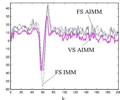
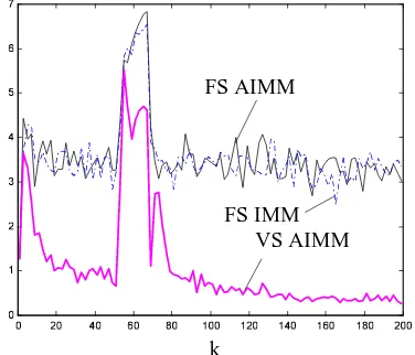
and the shortest response time. These inferences are confirmed by the mean error (ME) and the

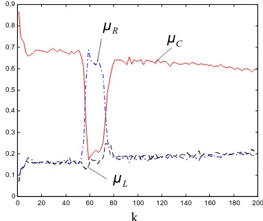
root-mean-square errors (RMSE) plots presented in Figs.2-4 and Figs.5-7. The average mode probabilities

are given in Figs.8-10. The ship moves at the beginning and at the end of the observed period uniformly, in the middle it makes a right turn that is reflected in the mode probabilities. The VS AIMM algorithm also provides the best and fastest model recognition. It is obvious from Figs. 11 and 12 that the above excellent VS AIMM algorithm performance is due to the self-adjustment mechanism for appropriate and timely control parameter tuning.

[image:13.595.314.505.75.236.2]

6. Conclusions

New models adequately describing the non-linear dynamics of manoeuvring ship motion are derived in the paper for the purposes of the manoeuvring ship tracking. A new variable-structure augmented IMM technique is also proposed. The designed ship models are implemented in a standard IMM and in the proposed here two augmented IMM algorithm versions with fixed and variable model structure. The proposed new AIMM algorithms use augmented state vectors and models to compensate the difference between the control parameters fixed in the IMM models and their current true values. Very good self-adjusting abilities are provided to the designed augmented IMM algorithms due to the estimated rate of turn. The accomplished extensive Monte Carlo simulation, shows that the VS AIMM algorithm outperforms the FS AIMM and FS IMM algorithms with respect to estimation accuracy and adaptability.

References

Abkowitz M. (1964): Lectures on Ship Hydrodynamics - Steering and Maneuverability.

—

HyA Rep.5.

Bar-Shalom Y., Ed. (1992): Multitarget-Multisensor Tracking: Applications and Advances, Vol. II.

—

Artech House, Inc.

Bar-Shalom Y. and X.R. Li (1993): Estimation and Tracking Principles, Techniques and Software.

—

Artech House, Inc.

Bar-Shalom Y. and X.R. Li (1995): Multitarget-Multisensor Tracking: Principles and Techniques.

—

Storrs, CT: YBS Publ.

Best R. and Norton J. (1997): A New Model and Efficient Tracker for a Target with Curvilinear Motion.

—

IEEE Trans. on AES, Vol.33, No.3, pp.1030-1037.

Ermolaev G. (1981): A Handbook of the Captain Sailing at Far Distances

—

Moscow, Transport (in Russian).

Farina A. and Studer F. (1986): Radar Data Processing, Vol.I.

—

J. Wiley & Sons.

Lerro D. and Bar-Shalom Y. (1993): Interacting Multiple Model Tracking with Target Amplitude Feature.

—

IEEE Trans. on AES, Vol.29, No.2, pp. 494-508.

Li X.R. (1996): Hybrid Estimation Techniques. In C.T.Leondes (Ed.), Control and Dynamic Systems, Vol.76.

—

Academic Press, NY.

Li, X.R. (1999): Engineers' Guide to Variable-Structure Multiple-Model Estimation, in Y. Bar-Shalom and W.D.Blair, eds., Multitarget-Multisensor Tracking: Advances and Applications, Vol. 3, Artech House.

Mazor E., Averbuch A., Bar-Shalom Y. and Dayan J. (1998): IMM Methods in Target Tracking: A Survey.

—

IEEE Trans. AES, Vol.34, No.1, pp.103-123.

Nomoto K. (1960): Directional Steerability of Automatically Steered Ship with Particular Reference to Their Bad Performance in Rough See.

—

DTMB Rep. 461, First Symp. on Ship Maneuverability.

Norrbin N. (1981): Theory and Observations on the Use of ARPA Mathematical Model for Ship Maneuvering in Deep and Confined Waters, SSPA No. 68.

Ogawa A. and Kayama I. (1977): MMG Report I, On Mathematical Model of Manoeuvring Motion of Ships.

—

Bulletin of the SNAJ, No. 575.

Pershitz R. (1973): Ship’s Maneuverability and Control.

—

Leningrad, Sudostroenie (in Russian). Semerdjiev E. and Bogdanova V. (1995): Nonlinear Model and IMM Tracking Algorithm for Sea

Radars.

—

Proc. of 40 Internation. Wissentschaftliches Kolloquim, Band 1, Ilmenau, Germany, pp.140-145.

Semerdjiev E. and Mihaylova L.(1998): Adaptive IMM Algorithm for Manoevring Ship Tracking.

—

Proc. of First International Conf. on Multisource-Multisensor Information Fusion, July 6-9, Las Vegas, USA, Vol.2, pp.974-979.

Sobolev G. (1976): Ship Maneuverability and Ships’ Control Automatization.

—

Leningrad, Sudostroenie (in Russian).