Storage and Security of Supply in the Medium Run

Munich Personal RePEc Archive

Storage and Security of Supply in the

Medium Run

Chaton, Corinne and Creti, Anna and Villeneuve, Bertrand

23 July 2008

Online at

https://mpra.ub.uni-muenchen.de/11986/

Storage and Security of Supply

in the Medium Run

Corinne Chaton

Anna Creti

Bertrand Villeneuve

July 23, 2008

Abstract

This paper analyzes the role of private storage in a market for a commodity (e.g. natural gas) whose supply is subject to the threat of an irreversible disruption. We focus on the medium term in which seasonality of demand and exhaustibility can be neglected. We char-acterize the price and inventory dynamics (accumulation, drainage and limit stocks) in a competitive equilibrium with rational expecta-tions. We show the robustness of our results to alternative scenarios in which either a disruption has finite duration or the crisis is foreseen. During the crisis consumers may put pressure on the Government to intervene, but too severe antispeculative measures would inefficiently discourage storage. Practical solutions to this dilemma cause welfare losses that we characterize and quantify.

∗_{Electricit´e de France R&D. E-mail: [email protected].} †_{Universit`a Bocconi-IEFE. E-mail: [email protected].}

1

Introduction

Natural gas consumption has grown fast in the European Union over the last decades. In 2005, about one-quarter of the EU primary energy consumption was based on natural gas, and imports from neighboring producers, mainly Russia, accounted for 35% of the total EU25 demand (DG TREN, 2006). Dependence on external supplies is going to increase in the next years, as gas consumption in Europe is expected to grow whereas indigenous sources are forecasted to slow down. This prospect raises serious concerns about security of supply.

What can be done? Pipelines and a diversified portfolio of long-term contracts with producers are the primary insurance against supply inter-ruptions. Security of supply targets can also be met by increasing system flexibility (fuel switching, interruptible contracts and liquid spot markets). However, these mechanisms have a limited capacity to absorb shocks such as extreme weather, technical breakdown, terrorism, which would endanger all the European countries at the same time and trigger a crisis (Weisser, 2007). In the short-medium term, precautionary gas storage is indispensable to ensure uninterrupted services in face of events of “low probability but high potential market impact” (Stern, 2004).1

The issue is a very complex one, so simplification is essential if any progress is to be made. We focus on the medium term in which both the seasonality of demand and the exhaustibility of gas can be practically ne-glected. All the agents know that there is a probability of an irreversible crisis. Storers are assumed to be risk-neutral and price-takers; they keep a stock of gas if expected price gains balance storage and interest cost. When the crisis occurs, the supply price jumps and the economy enters in a com-petitive Hotelling regime: storers gradually sell their stock and the price rises towards a ceiling, at which a stationary equilibrium is reached.

During the abundance phase, the anticipation of the crisis dynamics de-termines precautionary actions. The expected gains with respect to current prices provide a rationale for stockpiling. This stage is not trivial as we have to characterize a dynamic equilibrium consisting of both price and stocks trajectories. As long as the crisis has not hit the economy, accumulation starts fast and declines smoothly to approach but never reach limit stocks. Indeed, as time passes, storers become gradually cautious in their purchases and relieve pressure on the current price.

1

The basic insights of our analysis hold if we relax the irreversibility hy-pothesis, by analyzing crises of finite duration and foreseen supply disrup-tions. Thus the idea of a permanent supply shock, besides allowing explicit resolution of the model, is less restrictive than it would appear to be.2

Security of supply has an inevitable political dimension: consumers are reluctant to pay high prices in the crisis period and they put pressure on the Government to intervene. Stockholders may fear that if the consumers’ lobby prevails, antispeculative measures would dramatically decrease the capital gains they could expect. This might discourage storage completely. The Government has to find a practical solution to the trade-off between the costs of controlling prices and the benefits of strategic reserves. The resulting second best equilibrium inevitably creates welfare losses that we characterize and quantify.

Our approach is a useful complement to the models on oil supply security. We focus on the medium-term horizon analysis of the supply disruption, an issue that has been largely neglected in the works inspired by the theory of exhaustible resources.3 _{It is our opinion that this strand of the literature does}

not adequately represent the actual EU gas security of supply problem. Due to the high import dependence and the fast decline of internal gas production, it is unlikely that European countries are willing to further slow down the gas extraction rate in order to ensure future supply. Moreover, gas producers like Russia, Norway, Algeria do not seem to form a proper gas cartel.

Our work is related to Teisberg (1981), who developed a macroeconomic dynamic programming model. Our model shares with this paper the stochas-tic specification of the supply disruption. However, we put forth a rather dif-ferent perspective, since our model focuses on a microeconomic foundations (in particular arbitrage) to explain stocks formation and drawdown. This is also a noticeable difference with respect to Bergstr¨om et al. (1985) in which stocks are built up at the exogenous world price as they analyze the case of a “small country” that does not influence the international trade of the commodity exposed to an embargo threat.

Our analysis resembles the Wright and Williams (1982)’s approach in

2

Creti and Villeneuve (2007) develop an algorithm for solving a Markovian version of the present model in which the economy alternates between abundance and crisis. Though this latter approach may be deemed more realistic, its drawback is that most results are based on simulations.

3

that we derive the equilibrium dynamics of accumulation and drawdown in a continuous time context. Furthermore, like Williams and Wright (1991), we analyze welfare effect of public interventions. However, the assumption of i.i.d. shocks used by those authors cannot capture the persistence that supply crises are likely to exhibit. Moreover, in Williams and Wright, the complexity of the dynamic models makes the policy evaluation impossible to solve analytically. Our method, which uses only information on supply and demand fundamentals and the stochastic process, allows full description and evaluation of the trajectories of the economy.

The paper is organized as follows. Section2presents the dynamic model. Section 3 provides the characterization of the competitive equilibrium. We find equilibrium prices, limit stocks and drainage time. In Section 4, we show the robustness of our results to alternative scenarios in which either a disruption has finite duration or the crisis is foreseen. Section5is devoted to policy issues. To give useful orders of magnitude, we illustrate our method with parameters roughly calibrated on the UK gas market. We suggest in Section 6two important extensions of the basic model: non negligible injec-tion and release costs, and limited storage capacity. We conclude by pointing out that the methodology can be adapted to other commodities or regions. Proofs and technical results are relegated to the Appendix.

2

The model

The economy starts at date 0 in a state of abundanceAand passes irreversibly at a random date in a state of crisisC. Time is continuous. The probability that the economy switches fromAtoC in a time intervaldtisλdt,whereλis the publicly known parameter of this survival process. Thus, if the economy is in state A at some date, the economy will still be this state t periods later with probability e−λt_{. This simple modeling has three properties: (1)}

irreversibility ; (2) the crisis is certain only when it happens (no warning); (3) λ is independent of the state of inventories. The first two properties are relaxed in Section 4 whereas the third is kept throughout the paper.4 _In

any case, this structure represents the notion of low probability/high impact event (Stern, 2004).

We assume that consumers and producers only respond to the current price and the stateσ =A, C. These responses are summarized by the “excess

4

Since disruption risk linked with terrorist attack, civil war or pipeline breakdown can reasonably be seen as independent of accumulated reserves. Teisberg (1981) considers the deterrence effect of having sufficient reserves. However, the specification is givena priori

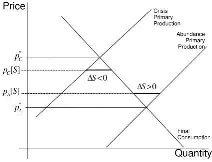
supply functions” ∆σ[·] defined over R∗₊, where ∆σ[p] is the difference in

state σ and for pricepbetween current primary production and currentfinal consumption. For example, ∆C[·] incorporates the supply shock and the

adaptation of demand to the new state (e.g. use of interruptible contracts, fuel switching).5

Excess supply function ∆σ[·] is increasing and has a unique finite positive

zero in R∗

+, denoted by p∗σ; this is the price at which the spot market would

be balanced without recourse to storage. Therefore, if the current price pis above p∗

σ, then the economy stores (∆σ[p] > 0); if p is below p∗σ, then the

economy draws on gas inventories (∆σ[p] < 0). Naturally, we assume that

the abundance static equilibrium price p∗

A is strictly smaller than the crisis

static equilibrium price p∗

C. See Figure 1 for an illustrative example.

∆σ[·] is a flow in the sense that if price p is sustained for the interval

dt, then the quantity that is stored is ∆σ[p]dt. Thus, if we denote the total

inventories in the economy by S ≥ 0, conservation of matter imposes the following conditions

dS

dt = ∆σ[p] if S >0 or ∆σ[p]>0, dS

dt = 0 if S = 0 and ∆σ[p]≤0.

(1)

Storers are assumed to be risk-neutral price-takers, so that the price dy-namics will be driven by arbitrage.6 _{Storage exhibits constant returns to}

scale. Carrying costs consist of the opportunity cost of capital (r being the interest rate) and a cost c (per unit of commodity and per unit of time).7

We define the equilibrium as follows.

Definition 1 A competitive equilibrium starts at date 0, in state A, with some initial stocks S0; it consists of contingent prices and stocks trajectories

{pA[t], pC[t, τ]}_t≥0,τ≥0 and {SA[t], SC[t, τ]}_t≥0,τ≥0 (2)

where t is the current date andτ the (random) date at which the crisis breaks out.

Three conditions must hold: (1) price-taking behavior by all agents (con-sumers, producers, storers); (2) rational expectations; (3) conservation of matter.

5

This modeling is rationalizable with agents maximizing intertemporal utility or profit, provided objectives are time separable and quasi-linear. For a full justification, see Ap-pendixA.4where surpluses are calculated.

6

We should rather write “quasi arbitrage”, since speculators break even in expectation only.

7

* C

p

0

S ∆ >

* A

p

Crisis Primary Production

Abundance Primary Production

Final Consumption

0 S

∆ <

[ ]

A

p S [ ]

C

p S

Price

Quantity

Figure 1: Supply disruption in the linear case.

The date of the crisis τ has no impact on pA[·] nor SA[·]; moreover pC[·]

andSC[·] are defined only for dates posterior to the disruption. Non-strategic

behavior of the agents, strictly increasing excess supply functions, linearity of the storage technology, risk-neutrality, all these hypotheses suffice to ensure that the competitive equilibrium is Pareto optimal.

3

Price and stock dynamics

Storers keep a stock of gas if expected price gains balance storage and interest cost. Whenever storages are non-empty, for a time increment dt, the no-arbitrage equations read

pC[t, τ] +cdt = (1−rdt)pC[t+dt, τ], t≥τ, (3)

pA[t] +cdt = (1−rdt) ((1−λdt)pA[t+dt] + (λdt)pC[t+dt, t]). (4)

In the above equations, the LHS is the unit price plus stockholding cost in states of crisis C and abundance A respectively. The RHS is the expected present unit value of the stocks after dt has elapsed. Equation (4) incorpo-rates the risk of a regime switch. After elimination of second order terms, we get

∂pC[t, τ]

∂t = rpC[t, τ] +c, t ≥τ, (5)

dpA[t]

We solve the model backwards. Once the crisis has broken out, the econ-omy follows the Hotelling (competitive) dynamics; the gas price increases and the stocks shrink. Equation (5) is integrated for a fixed dateτ and gives for all t≥τ:

pC[t, τ] = min

n

(pC[τ, τ] +

c

r) exp[r(t−τ)]− c r, p

∗ C

o

. (7)

The price stops atp∗

C when the precautionary reserves are exhausted. Indeed,

if the price were to overpass p∗

C, the economy would start accumulating gas

without bound or time limit, which cannot be an equilibrium.

The economy drains the stocks that were in place at dateτ,thus conser-vation of matter implies:

SC[t, τ] = −

Z +∞

t

∆C[pC[s, τ]]ds, (8)

SA[t] = S0+

Z t

0

∆A[pA[s]]ds, (9)

SA[t] = SC[t, t] for all t. (10)

None of the model’s parameters—interest rate, costs, crisis probability— depend on time. This simplifies the representation of the equilibrium, as the following proposition shows.

Proposition 1 The equilibrium prices are only functions of current stocks. FunctionspA[S]andpC[S]are continuous and decreasing for allS ≥0; pC[S]

has a simple implicit expression

S =−

Z p∗

C

pC[S]

∆C[p]

rp+cdp. (11)

By using the results of Proposition1and equation (7), we obtain drainage duration for stocks S:

D[S] = 1

rln

rp∗ C +c

rpC[S] +c

. (12)

This confirms that larger stocks always need more time to be drained. Drainage duration is necessarily finite: once the price has reached p∗

C, it would be

un-economical to keep costly stocks whose value will never increase.

The following proposition contains the fundamental properties of the equi-librium trajectories.

1. The maximum inventories during abundance S∗ _is

S∗

=−

Z p∗

C

pC

∆C[p]

rp+cdp, (13)

where

pC ≡

r+λ λ

p∗ A+

c

λ. (14)

S∗ _{is positive if and only if p}∗

C > pC. Moreover, S∗ verifiespC[S∗] =pC

and pA[S∗] =p∗A.

2. The protection offered to the economy by the stocks has a maximum duration

D∗

=D[S∗

] = 1

rln

λ r+λ

rp∗ C +c

rp∗ A+c

. (15)

3. When S∗ _{>0, the economy approaches S}∗ _{without reaching it.}

The price threshold and the limit stocks are remarkably useful to describe the behavior of the economy. During the state of abundance, storers are willing to pay a premium proportional to the expected capital gains. As stocks approach S∗_{, these gains are progressively eroded and storers relax}

their pressure on prices. Accumulation slows down so much that the limit stock is never attained.

The time length D∗ _{is positive if and only if S}∗ _{is positive. Maximum}

duration of drainage in equation (15) only depends on the boundary pricesp∗ C

and p∗

A, the interest rate and the unit cost. As a purely illustrative example,

let’s takecnegligible with respect to the opportunity cost of the stock (price times interest rate). Limit stock and drainage time are non null if:

p∗ C

p∗ A

> r+λ

λ . (16)

For instance, with an interest rate of 5% and a “one-in-twenty-years” crisis (λ = 5% approximately), equation (16) implies that some precautionary storage takes place if the ratio p∗

C/p ∗

A is larger than 2.

The impacts of parameters c, r, λ are unambiguous. With a higher unit storage cost or interest rate, the integrand in (13) decreases (the denominator increases) and the lower bound of integrationp_C increases, thusS∗ _decreases.

With a higher crisis probability, pC is smaller, which gives a larger S∗. The

4

Weakening the irreversibility hypothesis

In this section, we somewhat relax the irreversibility hypothesis by extending the model in two directions: first, we consider finite duration of the crisis, and second, we study the impact of “alerts” in the management of stocks.

Crisis of finite duration. The notion of excess supply function ∆C[·]

in-corporates the short-term reactivity of the economy to the shock via demand curtailment or fuel switching. Liberalized gas market also offer interest-ing possibilities to overcome disruption problems: the supply crisis can be solved by negotiating new contracts with gas producers and developing ad hoc transport infrastructure. Since these solutions entail long and complex procedures, a crisis may be of long but finite duration.

Assume that agents know that the crisis will last a period of lengthL, after which the economy returns to abundance. When L > D∗

, the accumulation and drainage dynamics behave as if the crisis were irreversible. If L < D∗_,

the limit stock, denoted by SL_{, is smaller than S}∗ _{and it increases with the}

crisis duration L; in fact when the crisis duration approaches the threshold

D∗ _{from below, the limit stock S}L _{goes to S}∗_{. If the shock occurs early,}

the accumulated stocks might be insufficient to last the whole duration of the crisis. If, in contrast, the economy has approached SL _{sufficiently, the}

price will pass from pC at the beginning of the crisis, as we saw earlier, to

a maximum value (pC + rc) exp[rL]− c r < p

∗

C at the end of the crisis which

coincides with complete stockout. Quite intuitively, storage is more effective at keeping moderate prices for short crises.

Alert and crisis. Assume that the crisis is announced (the “alert”) before

it happens. In the abundance state, an alert occurs with probability λdt in a time interval dt; after a delay of T time units, T being perfectly known, the disruption itself takes place. We could think of T as being a few weeks or months (up to now, everything was as if we had assumed T = 0).

There are two finite thresholds T and T with T < T separating the three different regimes that we are going to describe (see Appendix A.3 for calculations).

Assume that the date of the crisisτ has always been known. As stockpil-ing too early is not profitable, there is a unique T such that at date τ −T ,

the economy starts storing and does so until date τ; from then on, the stock is drained.

atp∗

A untilT time units before the crisis, and then grows continuously up to

p∗

C. In the transition, stocks are piled up during the alert and drained once

the crisis has hit the economy. A consequence of the increasing price is that accumulation accelerates as the date of disruption approaches, a remarkable difference with the basic model.

If T is slightly below T, the price of gas jumps as soon as the crisis is announced and storers accumulate until the crisis occurs. Quite intuitively, the jump increases as T shortens.

If T is small enough, the price just after the alert could jump to pC or

more if inventories were quasi empty. The threshold is denoted by T. Thus, if T < T (with 0< T < T), some accumulation takes place before the alert. In that case, accumulation can be broken down into two phases. Before announcement of the disruption, the stock converges towards a limit; during this phase, the price decreases smoothly towards p∗

A. The alert starts a new

phase in which the price jumps and increases until stocks are exhausted.

5

Dynamic welfare costs of antispeculative

policy

In theory, governments should not interfere with security of supply, as com-petitive markets realize efficient solutions (Bohi et al., 1996). However, the Government might pursue short term political goals, supported by the con-sumers’ pressure groups demanding stable supply of energy at an affordable

price, no matter what the circumstances are (Mulder and Zwart, 2006). In view of this, storers would anticipate strict price controls.8 _{Given the}

dis-couraging effects of this threat, the Government may wish to mitigate in advance its own foreseeable antispeculative intervention.9 _{Our objective is}

to quantify the welfare loss of such second best policies.

The result of this political process can be summarized in terms of our model as follows. The policy consists of an “antispeculative” price pG

C which

8

As Wright and Williams (1982) put it: “the oil industry has abundant reason to believe that there is some oil price at which Government will intervene to control the realizations of oil drawn down from private storage in times of shortage, when profit-maximizing private storers and importers may well be branded as “speculators” or “price gougers”. In fact, it may well be impossible for any administration credibly to guarantee against such action by itself or its successors.”

9

is smaller than p∗

C and independent of S for clarity. It is the price at which

gas is sold and purchased as long as there are stocks to be drained. Since pG C

induces a fixed drainage rate ∆C[pGC], the price pGC is guaranteed for a fixed

period only. From then on, stocks stay empty and the price is p∗

C. Since

storing during crisis yields negative returns (the price cap prevents capital gains), storers sell all they have as soon as the crisis starts. To accommodate this, the Government can establish a public stabilization fund, which may either directly manage storage, or remunerate owners of storage facilities for their services, or pay stockholders their opportunity cost. All these schemes are equivalent as they engender the same surplus in total, though they differ as for how it is distributed across actors.

There are two cases, leading to very different equilibrium outcomes. If the crisis controlled price pG

C is expected to be below pC, the smallest price that

makes stockholding profitable, storage is totally discouraged in the abun-dance phase. If, on the contrary,pG

C is abovepC, storers see it as a price floor

and they will not stop accumulation on their own in the abundance phase. Any inventory level can be attained if the crisis occurrence lags. To avoid this distortion, the Government has to put an upper bound on gas invento-ries, denoted by SG_{. Here two variations are possible: either the abundance}

price is endogenous or it is also controlled by the Government. We take the second option. Indeed, ifpG

A were determined by the market,

arbitrage would make it equal to λ r+λp

G

C − r+cλ all along the accumulation

phase. The stabilization fund established by the Government can replicate this price, hence our approach may deemed rather general. Moreover, the theory of the second best says that pG

C being distorted by political pressure,

pG

A may be voluntarily distorted by the Government: along withSG,pGAserve

to mitigate post crisis inefficiencies generated by the price cap.

To evaluate the antispeculative policy, we calculate the expected present surplus based on generated price and stocks trajectories. This yields a func-tion of S, the stocks at the date the value is computed. Welfare being determined up to some arbitrary constant, we normalize our comparisons by setting at zero the value of the counterfactual no-storage policy (as if storage were impossible or too costly).

We denote the value of the optimal policy by V∗

A[S] and the value of

the antispeculative policy by VG

A[S]. The following index measures welfare

performance:

v = V

G A[S]

V∗ A[S]

. (17)

resources by, e.g., building exaggerated stocks too fast and by using them too timidly. Such examples are (unfortunately for the society) quite easy to find as we shall see.

The detailed calculations of the total expected present surplus and of the index in equation (17) are relegated to Appendix A.4.

Linear model. The application assumes linear excess supply functions:

∆C[pC] =bpC−a ; ∆A[pA] =βpA−α. (18)

The reference prices are p∗

C = a/b > p ∗

A = α/β. Figure 1 illustrates the

supply disruption in the linear case. We compare now the two scenarios:

1. Competitive/surplus maximizing scenario;

2. Antispeculative policy summarized by pG

A, pGC, SG

.

The surplus maximizing limit stockS∗ _{and drainage timeD}∗_{have explicit}

formulas that are calculated by using equations (13) and (15) respectively.10

Moreover, pC[S] can also be calculated, whereas pA[S] and VA∗[S] are solved

numerically.

To give realistic orders of magnitude, we take parameters as roughly cal-ibrated on the 2006 UK gas market. The UK having recently moved from a position of relative self-sufficiency to one of import-dependence, the need to implement precautionary gas stocks has been debated and much data have been released (see Appendix A.5 for details).

In Figure 2(a), we show prices as a function of the stocks. Figure 2(b) depicts accumulation and drainage for alternative scenarios.11

Accumu-lation starts at date t = 0 with S = 0 and the shock occurs at dates

t = 10,20,· · ·,80. During the abundance phase, stocks are gradually piled up to approach S∗ _{= 7.7 and the price decreases toward p}∗

A = .6. When

the crisis hits the economy, the price jumps to pC[S] and increases toward

p∗

C = 12. Though it can take as long as D

∗ _{= 5.4, drainage appears as much}

faster than accumulation.

10

The limit stock is

S∗=bc+ar

r2 ln

λ

r+λ

rp∗C+c

rp∗

A+c

+b

r

r+λ

λ p

∗

A+c

−p∗C

. (19)

The expression forD∗ _{involves Lambert’sW function, the inverse off(w) =we}w_.

11

2 4 6 2

4 6 8 10 12

S

[ ] C

p S

[ ] A

p S

Price

20 40 60 80

1 2 3 4 5 6 7

t S

(a) Equilibrium price functions. (b) An array of stocks trajectories.

Figure 2: The equilibrium prices and trajectories.

As for the second best policy, we numerically calculated the surplus maximizing antispeculative storage.12 _{We found p}G

A = .84, p G

C = 10.5 and

SG _{= 4.9. Accumulation takes 21.4 years, if no crisis breaks out before;}

drainage itself takes a maximum of 3.4 years.

Welfare comparison. Figure 3(a) displays the relative value v of the an-tispeculative policy. Over the interval [0,4.9) where both surplus are defined, the index approaches 1 as inventories S increase:

• AtS = 0, the suboptimal policy achieves 86% of the potential surplus;

• Gains increase very fast at the beginning of accumulation: at S = 1 (that is 20% of SG_{), 64% of the initial efficiency loss are recouped;}

• At SG_{, 95% of the maximum surplus are captured by the suboptimal}

policy.

The latter effect is easily explained: as storage increases, the inefficiency of the accumulation strategy is sunk and thus disappears from the welfare comparison.

The expected present surplus is quite sensitive to the chosen policy. An simple example of a policy that dramatically underperforms the no storage option is proposed. Assume that the Government keeps SG _{as a target but}

imposes a twice larger accumulation rate and a twice slower drainage rate than those obtained under the surplus maximizing antispeculative policy.

12

VG

A[0] can be expressed as an explicit function of constrained prices and target stock

(pG A, p

G C, S

G₎

1 2 3 4 5 0.88

0.9 0.92 0.94

S

v

1 2 3 4 5 6 7

-0.6 -0.4 -0.2 0.2 0.4

SS

S

v

(a) Constrained optimum. (b) Alternative.

Figure 3: Relative value of suboptimal policies.

As Figure 3(b) shows, at zero stocks and up to S = 1.4 approximately, the policy imposes huge welfare costs (the index starts at −.72). This means that the economy would be better off if storage were impossible. Due to fast accumulation, the price is very high during the accumulation phase, which penalizes consumers; in addition, the economy sustains the cost of excessive reserves. This effect becomes attenuated as storage expenditures get sunk, but to a much lesser extent than with the constrained optimum.

6

Extensions

Injection and release costs. The analysis can be easily extended to the case where the costs of injecting and releasing gas are non negligible. Denote unit injection cost byiand unit release cost by s. With perfect competition, gas outside and inside the reservoir state can be traded at prices that we denote respectively by pσ[S] and pIσ[S] (with σ = A, C and S ≥ 0). The

market equilibrium between outside and inside gases implies that, whenever

S > 0,

pA[S] +i=pIA[S] and pC[S] =pIC[S] +s. (20)

The structure of the system of equations is preserved, with pI

σ replacing pσ.

Arbitrage conditions (27) and (28) become

∆C[pIC+s]·

dpI C

dS = rp

I

C +c, (21)

∆A[pIA−i]·

dpI A

dS = (r+λ)p

I A−λp

I

Remark that the excess supply functions are shifted, thus boundary condi-tions are

pI

C[0] = p ∗

C −s, (23)

pI A[S

∗_{] = p}∗

A+i. (24)

The range of pI

σ is narrower than that of pσ: the minimum is higher, the

maximum is lower. As a result, the condition ensuring positivity of the limit stock is more restrictive, i.e.

p∗

C −s >

r+λ λ

(p∗

A+i) +

c

λ. (25)

Expressions of optimal limit stock and drainage time are now based on shifted excess supply functions and shifted boundary prices.

Limited storage capacity. Gas is mostly stored in depleted fields and aquifers; the development of such facilities is naturally limited. If the capacity devoted to precautionary storage K exceeds S∗ _{previously calculated, then}

the unconstrained solution remains valid; otherwise, the maximum stock is constrained to equal K,which in turn affects price trajectories and the value of storage facilities.

During the crisis,pC[S] is unchanged compared to the unconstrained case.

Reserves are gradually drained, meaning that the storage price, under com-petitive assumption, remains fixed at the marginal cost c. In the abundance state, the price functionpK

A[S] depends onK: the accumulation process must

stop when capacity is saturated, therefore pK

A[K] =p ∗

A. The storage price is

also cas long as some capacity remains vacant; whenK is attained, it jumps to πK

A > c, with

πK

A =λ(pC[K]−p∗A)−rp ∗

A. (26)

The net rentπK

A−c, captured by the owners of the storage capacity, balances

the carrying costs of a fixed stock with its expected benefits. Storage capacity units gain value as K diminishes. This combines two effects: the smaller

K becomes, the larger πA, and also the shorter the time before saturation

will be. The first effect (the monotonicity of πA) derives directly from the

monotonicity of pC[K]. The second effect is shown in Appendix A.6.

7

Conclusion

trajectories, accumulation and drainage behavior are interdependent in equi-librium. This differentiates the approach from inventory management models in which prices are given, or precautionary reserve studies in which the wel-fare costs of building the stocks are ignored.

We found results that might prove useful not only in the context of the gas industry, but also for all those primary commodities whose market is ex-posed to a supply disruption threat. A simple condition determines whether precautionary stocks should be accumulated. General cost structures, in par-ticular limited storage capacity, or a richer timing of the crisis occurrence are shown to have intuitive and calculable effects on the main properties of the equilibrium. The impact of expropriation threats that discourage storage can be dramatic. Our insights into politically sustainable solutions could be easily transposed to other examples or market structures beyond the specific application we have analyzed.

A

Appendix

A.1

Proof of Proposition

1

The RHS of (8) is strictly increasing in the value of pC[τ, τ], thus it gives a

unique strictly decreasing relationship between pC and S ≥ 0, denoted by

pC[S]. We can then definepA[S] by backwards induction.

We can now replace the price dynamics in (5) and (6) by

∆C[pC[S]]·

dpC[S]

dS = rpC[S] +c, (27)

∆A[pA[S]]·

dpA[S]

dS = (r+λ)pA[S]−λpC[S] +c, (28)

for S > 0.

Equation (27) can be integrated directly to get equation (11). The RHS of (28) cannot be positive (otherwise storers would liquidate inventories at once) implying that dpA[S]

dS <0.

A.2

Proof of Proposition

2

1. Remark that pC is the minimum value pC[·] can take: storers are just

indifferent between keeping or selling their stocks if the abundance price is as low as p∗

A, since the carrying costs (rp ∗

A+cper unit) equals the expected

earning (λ(pC[S∗]−p∗A) per unit). The corresponding stocks are denoted by

S∗_{; S}∗ _{being the maximum stocks, it verifies p}

This reasoning implies in particular that ifpC ≥p∗C, thenS∗ = 0: holding

inventories cannot be profitable and the crisis will simply cause a price jump from p∗

A top∗C.

2. By plugging pC into (11), we obtain the expression in the text.

3. The pricepA must converge continuously towardsp∗Abefore the

occur-rence of the gas disruption. AspAcovers half its difference with the limitp∗A,

the variation rate of the stock per unit of time ∆A is approximately halved

(the derivative of excess demand atp∗

Ais not zero), meaning that the

conver-gence speed dS/dt is approximately halved. This implies that, whatever the proximity of the limit, the duration to cover half the distance to the limit is approximately constant, thus the limit is not attained in finite time.

A.3

Alert duration thresholds

Derivation ofT . Assume thatT is large. Once the economy is in alert, un-certainty vanishes and the price passes continuously from p∗

A top ∗

C following

the differential equation

dp

dt =rp+c. (29)

Letp∈(p∗

A, p∗C) be the price reached when the crisis occurs. Using the same

change of variable as in the text, we know that conservation of matter implies

Z p

p∗

A

∆A[p]

rp+cdp+

Z p∗

C

p

∆C[p]

rp+cdp= 0. (30)

p is unique since both terms increase as p increases, whereas the LHS is negative for p=p∗

A and positive for p=p∗C.

T is the time required for the price to pass from p∗

A top, i.e.

T = 1

rln

rp+c rp∗

A+c

. (31)

Derivation of T . For all T between T and T, the immediate post-alert price pT

A must be such that, prior to alert, storage is not profitable, i.e.

pTA< pC. (32)

Letp_ebe the price of gas at the instant the crisis occurs; it is uniquely defined by the conservation of matter equation

Z ❡p

pT A

∆A[p]

rp+cdp+

Z p∗

C

❡

p

∆C[p]

Given the price dynamics, the time Te required for the price to pass from pe

to p∗ C is

e

T = 1

rln

rp∗ C +c

rpe+c

. (34)

Thus Te decreases when peincreases, which implies in turn that the quantity to be drained is decreasing w.r.t. p_e(drainage time is an increasing function of the inventories).

To accumulate these smaller stocks, the price finishes higher in the abun-dance phase (last accumulation price isp_e, meaning that this phase of duration

T has to be shorter whenpeincreases). Given thatT is the time to pass from

pT

A to pe,pTA has to increase.

We conclude that T decreases as pT

A increases in the interval [p ∗

A, pC]. In

particular that pT

A=p∗A and p T

A=pC, thus T < T.

A.4

Expected present surplus

Consider a representative consumer whose intertemporal utility function val-orizes gas consumption and a separable num´eraire. Leaving aside uncertainty at this stage, the consumer’s objective can be written as

+∞

Z

0

(uσ[qt]−ptqt)e−rtdt, σ =A, C, (35)

where uσ is a state dependent, increasing and concave utility, qtis date t gas

consumption and ptqt is date t expenditure. Consider also a representative

producer whose technology can by aggregated at t by a state dependent convex cost function Cσ[qt].

For a given price p, final demand is u′−1

σ [p] and primary production is

C′−1

σ [p], thus excess supply functions as we defined them can be expressed

∆σ[p] =Cσ′−1[p]−u ′−1

σ [p]. (36)

The instantaneous surplus depends only on the stateσ,S and the current price p

Wσ0 +Wσ[p]−cS (37)

whereW0

σ denotes thereference surplus, i.e. calculated at pricep∗σ,and where

cS is the cost of keeping the inventories. The key point is that Wσ[p] can be

derived from the excess supply function ∆σ[p]:

Wσ[p] =

Z p

p∗_σ

Abundance Primary Production

Final Consumption

Lost consumer surplus Extra production cost Substracted -- -* A p p Price Quantity

Not in picture: −cS

Crisis Primary Production

+ +

Extra consumer surplus Saved production cost Added + * C p p Final Consumption

Not in picture: −cS

Price

Quantity

(a) Abundance state. (b) Crisis state.

Figure 4: Instantaneous surpluses in abundance and crisis states.

as we can directly see in Figure 4.

The final step consists of calculating the expected present surplus, by dis-counting all future instantaneous surpluses and then taking the expectation. Given the initial state A, stock S0 at date 0 and the stockholding dynamics,

the expected intertemporal surplus of the optimal policy is denoted:

V_A0+V∗

A[S0], (39)

where V0

A is defined as

VA0 =

W0

A

r+λ +

λW0

C

r(r+λ), (40)

and

V∗

A[S0] =E

   +∞ Z 0

Wσt[p

∗

σt[St]]−cSt

e−rt_dt

 

, (41)

σt being the (random) state at date t.

The antispeculative policy (summarized by pG

σ and constrained

accumu-lation and drainage functions ∆σ[pGσ]) will generate the instantaneous surplus

W∗

σ +WσG[pGσ]−cS. Total expected present surplus is:

VA0+V G

A[S0], (42)

where V0

A is defined by (40) and

VG

A[S0] =E

   +∞ Z 0

Wσt[p

G

σt]−cSt

e−rt_dt

 

The Bernoulli process driving the evolution of σt being exogenous and

time independent, the terms comprising W0

A and WC0 are identical whatever

the policy evaluated and therefore V0

A can be normalized at zero. This is

why we state that the no storage policy (a useful reference) can be given null value. The relative value of a given policy with respect to the optimum is therefore correctly captured by the index:

v = V

G A[S]

V∗ A[S]

. (44)

A.5

Calibration on UK data

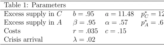
To calibrate our model, we take the following parameters values:

Table 1: Parameters

Excess supply in C b=.95 a= 11.48 p∗ C = 12

Excess supply in A β =.95 α=.57 p∗ A =.6

Costs r=.035 c=.15 Crisis arrival λ=.02

Time unit is the year, prices are in£_{/therm (1 therm = 2.76 m}3_),

quanti-ties are expressed in billion therm. As for the probability of crisis (λ=.02), we consider the value that DTI (2006, p. 90) estimates as a “realistic chance of a significant supply interruption”, based on ILEX (2006), JESS (2006), Ox-era (2006) reports. The interest raterand the maximal crisis price (a/b= 12) is taken from ILEX (2006, p. 106).13 _{The average 2006 price (α/β =.6) and}

annual consumption (about 36 billion therm) is documented by DTI (2007). The marginal cost of storage c is evaluated from available information, re-leased by Centrica Storage Ltd, on the largest UK storage facility. Missing parameters are calculated with identifying assumptions: in case of major crisis, consumption could be reduced by 30% (price 12, inventories release notwithstanding). Finally we adopt a last (arbitrary) condition: b=β.

A.6

Monotonicity of the scarcity rent

The functionpK

A follows ODE (28), with boundary conditionpKA[K] =p∗A.As

the function pC is independent of K, the Cauchy-Lipschitz theorem implies

that the price functions for two different capacities below S∗ _{never cross.}

13

Thus for all S ∈ [0, K] and K < K′_{, p}K

A[S] < pK

′

A [S] with both functions

decreasing. We now show that the timeTK needed for the price to pass from

pK

A[0] to p∗A is longer the larger is the capacity K. Using equation (28), we

have

TK =−

Z pK A[0]

p∗

A

dpA

(r+λ)pA−λpC[p K(−1)

A [pA]] +c

. (45)

Given the monotonicity of pK

A with respect toK,the above sum with a larger

K integrates a function of higher absolute value over a longer interval. This gives us the announced result.

References

Bergstr¨om, Clas, Glenn C. Loury and Mats Persson (1985), “Embargo Threats and the Management of Emergency Reserves,” Journal of Po-litical Economy, 93(1), 26-42.

Creti, Anna and Bertrand Villeneuve (2008), “Equilibrium Storage in a Markov Economy.” Available at:

http://83.145.66.219/ckfinder/userfiles/files/pageperso/bvilleneuve/Markovian.pdf

Crawford, Vincent, Paul Joel Sobel and Ichiro Takahashi (1984), “Bargain-ing, Strategic Reserves, and International Trade in Exhaustible Re-sources,” American Journal of Agricultural Economics, 66(4), 472-80.

Devarajan, Shantayanan and Robert J. Weiner (1989), “Dynamic Policy Co-ordination: Stockpiling for Energy Security,” Journal of Environmental Economics and Management, 16(1), 9-22.

DG TREN (2006), Statistical pocketbook, Brussels.

DTI (2006), “The Energy Challenge,” London.

DTI (2007), “Energy Market Outlook,” London.

JESS (2006), “Long-Term Security of Energy Supply,” Report to DTI, Lon-don.

Hillman, Arye L. and Ngo Van Long (1983), “Pricing and Depletion of an Exhaustible Resource when There is Anticipation of Trade Disruption,” Quarterly Journal of Economics, 98(2), 215-233.

Hogan, William (1983), “Oil Stockpiling: Help Thy Neighbor,”Energy Jour-nal, 4(3), 49-71.

Hughes Hallett, A.J. (1984), “Optimal Stockpiling in a High-Risk Commod-ity Market: The Case of Copper,”Journal of Economic Dynamics and Control, 8(2), 211-238.

ILEX (2006), “Strategic Storage and Other Options to Ensure Long-Term Security of Supply,” Report to DTI, London.

International Energy Agency (2003), World Energy Investment Outlook, Paris.

Mulder, Machiel and Gijsbert Zwart (2006), “Market Failures and Govern-ment Policies in Gas Markets,” CPB Memoranda 143, CPB Nether-lands Bureau for Economic Policy Analysis.

Nichols, Albert and Richard Zeckhauser (1977), “Stockpiling Strategies and Cartel Prices,” Bell Journal of Economics, 8(1), 66-96.

Oxera (2007), “An Assessment of Potential Measure to Improve Gas security of Supply,” Report to DTI, London.

Stern, Jonathan (2004), “UK Gas Security: Time to get Serious,” Energy Policy, 32(17), 1967-1979.

Stiglitz, Joseph (1977), “An Economic Analysis of the Conservation of De-pletable Natural Resources,” Draft Report, IEA, Section III.

Sweeney, John (1977), “Economics of Depletable Resources: Market Forces and Intertemporal Bias,” Review of Economic Studies, 44, 125-142.

Teisberg, Thomas J. (1981), “A Dynamic Programming Model of the U.S. Strategic Petroleum Reserve,” Bell Journal of Economics, 12 (2), 526-546.

Weisser, Hellmuth (2007), “The security of gas supply—a critical issue for Europe?,” Energy Policy, 35(1), 1-5.

Williams, Jeffrey C. and Brian D. Wright (1991): Storage and Commodity Markets, Cambridge University Press.