Munich Personal RePEc Archive
Lifetime Network Externality and the
Dynamics of Group Inequality
Kim, Young Chul
Korea Development Institute
1 May 2009
Online at
https://mpra.ub.uni-muenchen.de/18767/
Lifetime Network Externality and the Dynamics of Group Inequality
(Job Market Paper)
Young Chul Kim∗†
Brown University
February 2, 2009
Abstract
The quality of one’s social network significantly affects his economic success. Even after the skill acquisition period, the social network influences economic success through various routes such as mentoring, job searching, business connections, or information channeling. In this paper I propose that a social network externality which extends beyond the education period – what I call a Life-time Network Externality – is important in explaining the evolution of between-group inequality in an economy. When the members of a group believe that the quality of their social network will be better in the future, more young group members invest in skill achievement because they expect higher returns on investment realized over the working period. As this is repeated in the following generations, the quality of the group’s network improves over time. Combining the Life-time Network Externality, which operates during the labor market phase of a worker’s career, with the traditional concepts of peer and parental effects, which operate during the educational phase (Loury 1977), I suggest a full dynamic picture of group inequality in an economy with multiple social groups. I define a notion of Network Trap, wherein a disadvantaged group cannot improve the quality of its network without a governmental intervention, and I explore the egalitarian poli-cies to mobilize the group out of this trap. This social capital approach suggests a positive effect of equality on economic growth in later stages of economic development and a positive effect of inequality in the early stage of economic development, consistent with Galor and Zeira (1993). Unlike the previous literature, the conclusion is derived without imposing the standard assump-tion of credit market imperfecassump-tions. Therefore, this implies that equality, by helping disadvantaged groups to move out of the network trap, has a positive effect on economic development even in a ma-tured economy without binding credit constraints, or in a society with public provision of schooling.
Keywords: Lifetime Network Externality, Group Inequality, Network Trap, Social Capital, Economic Development.
∗I am deeply indebted to my main advisor Glenn Loury for his thoughtful guidance and continual encouragement for
this project. I am highly obliged to Oded Galor, Kenneth Chay and Rajiv Sethi for valuable comments and suggestions for the improvement. I benefited greatly from discussions with Andrew Foster, Jung-Kyu Choi, Woojin Lee and Yeon-Koo Che, and comments from the participants of Applied Microeconomics Seminar and Race and Inequality Workshop at Brown University. Financial support from Brown University Merit Dissertation Fellowship and J. William Fulbright Fellowship is gratefully acknowledged. All remaining errors are mine.
1
Introduction
The acquisition of human capital occurs within a social context, and can be facilitated by access to the
right social networks. This paper examines one mechanism by which such social network externalities
affect the evolution of economic inequality between social groups.1 The interaction between network externalities during the education period and during the working period produces a unique dynamic
structure for the evolution of group inequality. The education period network externalities operate
as a historical force that restricts a group to be subject to the current network quality, while the
working period (or lifetime) network externalities operate asa mobilization force that leads a group to
enhance (or shrink) the skill investment activities by holding an optimistic (or pessimistic) view about
the future network quality. In the model to follow I identify what I will call the Network Trap, in
which the human capital development of a social group is trapped by the externality of social networks.
Also, I examine possible egalitarian policies to mobilize a disadvantaged group out of the trap and
improve its skill investment activities. Considering that human capital is a prime engine of economic
growth in the modern economy, I describe the macroeconomic effects of group inequality on economic
development (Loury 1981, Galor and Zeria 1993). The model I create finds a positive effect of equality
on the economic growth in most developmental stages. Unlike the previous literature, this conclusion
is derived without imposing the standard assumption of imperfect credit markets. Therefore, the
model implies a positive effect of equality even in an economy with no credit constraints: equality, a
more equal distribution of social network capital in this study, has a positive effect on the economic
development, by helping the disadvantaged groups to move out the network trap and enhance the skill
investment activities, even in the society with public provision of schooling.
Lifetime Network Externality
Socioeconomic disparities between social groups constitute a challenge in many countries around
the world. Even though social groups may educate their children within an identical educational
system and work in the same market economy, their skill achievement ratios and wage levels can be
significantly different. It is hard to conceive of a single root cause of inequality between groups since
the manner in which social groups are formed is unique to each society. For instance, groups form
along racial line in societies such as the Unites States, South Africa, New Zealand and Australia, but
form along religious lines in Turkey, Iraq, Pakistan, Northern Ireland and Israel. While ethnicity is
1Another approach to explaining group inequality explores the discrimination story: either taste-based discrimination
important in some countries such as Singapore, Indonesia, and the Balkan states, we often see caste-like
social division in India and Gypsies in Europe. In many western countries, the population is divided
into immigrants and non-immigrants, while population in the Americas is divided into indigenous
peoples and European descendants.2
Even though these cases are distinct from one another, a salient feature of the issue is consistent
throughout all the cases: divided social interactions between groups occurs over the whole lifetime.
The social network externality around the skill acquisition period and the consequent development
bias has long been discussed since the pioneering work of Loury (1977). In his theory, a human being is
socially situated in that familial and communal resources explicitly influence a person’s acquisition of
human capital through various routes, including the constraints of training resources, of nutritional and
medical provision, of after-school parenting, of peer effects, of role models, and even of the psychological
processes that shape one’s outlook on life.3 A number of subsequent theoretical works discussed the development bias, emphasizing the network externalities over the skill acquisition period, including
Akerlof (1997), Lundberg and Startz (1998) and Bowles, Loury and Sethi (2007).4 However, the
theoretical work continues to confront some empirical evidence that it cannot fully embrace. Consider
a few examples:
1. Over the industrialization process of South Korea in the 1970s and 1980s, the socioeconomic
disparity between Youngnam and Honam regional groups increased significantly, even when the
educational system was strictly based on the public provision of schooling, and when the familial
and communal environment did not carry a big difference between two regional groups: both
groups were in an early stage of development, poor and low skilled, and shared a similar cultural
base. It is often argued that social connections and mentoring networks played a key role in the
emergence of group disparity in South Korea (Ha 2007, Kim 2002).
2. In France, where the public school system is well established, the violence of second generation
immigrant youth in 2005 caused nearly 9,000 cars to be torched and dozens of buildings damaged
in a riot. Most of the rioters were unemployed youth who arguably suffered from social exclusion
2Also, groups have formed along linguistic lines in nations such as Canada, Switzerland, and South Africa
(Anglo-African and Afrikaners). Region of family origin influences the social interactions in nations such as Spain, the United Kingdom, and South Korea (Youngnam, Honam).
3His theory is supported by numerous empirical work, which includes the peer influence (Anderson 1990), community
effects (Cutler and Glaeser 1997, Weinberg et al. 2004), racial network effect (Hoxby 2000, Hanusheck, Kain and Rivkin 2002) and academic peer effect (Kremer and Levy 2003, Zimmerman and Williams 2003).
4Akerlof (1997) provides a theoretical argument, which states that concerns for status and conformity are the primary
in French society, and from the lack of a job network.
3. In his examination of the jobless black underclass in New York City, Waldinger (1996) concludes
that black unemployment originates from the lack of access to the ethnic networks through which
workers are recruited for jobs in construction and service industries.5
These examples illustrate the importance of social network externalities that operate beyond the
edu-cation period – what I am calling the Lifetime Network Externalities. This effect has been emphasized
in numerous empirical papers in the economics and sociology literature. The sociologist Granovetter
(1975) has been one of the pioneers of this line of inquiry. His work sheds light on the role played by
interpersonal relationships, such as friends and relatives, in channeling information about jobs and job
applications. He and other researchers have found that approximately fifty percent of all workers
em-ployed found their jobs on the basis of recommendation and word-of-mouth (Granovetter 1973, Myers
and Shultz 1951, Rees and Shultz 1970, Campbell and Marsden 1990).6 The role of ethnic networks in job search is emphasized in numerous empirical work such as immigrants in Australia (Mahuteau
and Junankar 2008), Mexican immigrants in the US (Livingston 2006 and Munshi 2003) and migrants
to urban centers in India (Banerjee 1981, 1983).7 The effects of social network go beyond just finding
jobs. Friends and acquaintances of the same occupation may help workers to increase productivity
and decrease the psychological stress of maintaining the occupation. Empirical papers show that a
worker with richer social networks can be more efficient in contacting business partners (clients and
customers) and handling specific work troubles (Fafchamps and Minten 1999, Laband and Lentz 1995,
1999, Falk and Ichino 2005, Khwaja e al. 2008). The mentoring effects of the social network can help
to increases job satisfaction, to minimize the turnover rate (Rockoff 2008, Castilla 2005, Cardoso and
Winter-Ebmer 2007, Bilimoria et al. 2006), and to heighten the recognition of opportunities in the
5In the postwar era of New York, the manufacturing industries where the blacks occupied jobs moved out or eroded
while the job opportunities in the service sector continued to grow with whites moving out of the sector. The immigrants who entered the low skilled service sector expanded their economic base through the ethnic networks, while the native blacks left behind jobless. Given employers’ preference for hiring through networks, information about job openings rarely penetrated outside the immigrant groups (Waldinger 1996). This empirical evidence brings a very different perspective from the spatial mismatch hypothesis (Kain 1968, Raphael 1998, Ross 1998), which insists that blacks in central cities lost jobs as employment moved to suburbs. The case in New York City reveals that blacks lost jobs even when whites moved out leaving jobs for minorities in the cities.
6Other researchers concludes that, among many different job search methods, personal connection of friends or
relatives is most widely used among unemployed youth in the US (Holzer 1987,1988, and Blau and Robins 1990), and in the UK (Gregg and Wadsworth 1996) and in Egypt (Assaad 1997, Wahba and Zenou 2005): Holzer (1988) finds 85.2% of jobseekers used friends/relatives ties, 79.6% used direct application without referral, 53.8% used state agency, and 57.8% used newspaper advertisement.In their study, the acceptance rate of job offers obtained through personal connection is highest (eg. about 82 percent in Holzer (1988)), implying that job offers through personal connection generally have higher wages or more appealing nonwage characteristics.
7Observing the evidence, Montgomery (1991) constructs a theoretical model that explains why firms hiring through
entrepreneurial process (Ozgen and Baron 2007). The empirical work suggests that the better the
quality of one’s social network, the higher the benefits one can expect, and, consequently, the more
incentive one has to invest in the acquisition of skills.
Dynamic Structure of Group Inequality
We conclude that both kinds of externalities – those operating during the education period and
those at work over the course of a worker’s lifetime – affect a social group’s overall skill investment
rate.8 As mentioned, this paper explores the dynamic structure of group inequality generated by the interaction between these two types of network externalities. These two effects operate via different
channels. With the education period network externality, change in a group’s status tends to be
subject to the “past”: by altering skill investment cost, the current stock of network human capital
directly affects the investment rate in a newborn cohort. By contrast, with the lifetime network
externality, change in a group’s status tends to be subject to the “future”: by altering the future
benefits anticipated to accrue from skill acquisition, the expected success of one’s network influences
skill investment in an entering cohort.
This latter effect implies a unique feature of the dynamic structure: the possibility of workers acting
together to improve, or deteriorate, the quality of a group’s social network. For instance, suppose that
a group’s network quality is relatively poor, but that a newborn cohort happens to believe the quality
of group’s network will be better in the future. If this belief leads more newborn group members to
acquire skills, then the next newborn cohort will find the overall network quality has improved because
of the enhanced skill investment of the previous cohort. If the next newborn cohort, and the following
cohorts, continue to hold the optimistic view of the future, they will keep the enhanced skill investment
rate and the quality of group’s social network will improve over time thereby justifying the optimistic
beliefs of earlier cohorts. However, suppose that the newborn cohort held a pessimistic view that the
network quality will be even worse in the future. Fewer members of the newborn cohort will invest in
the skill achievement because the expected benefits have declined. As the following cohorts continue
to hold the pessimistic view, the network quality will be deteriorated over time. So, this pessimistic
belief could also be self-fulfilling.
However, collective action to influence such beliefs may not be feasible for all social groups with
unequal network quality. The potential impact of altering beliefs is restricted by the strength of
education period network externalities. That is, collective action through optimism or pessimism
cannot play any role when the quality of network is too good or too bad.9 Therefore, the analysis
8For example, when a group’s social network contains more highly skilled members, then more of its newborns will
invest in skills – not only because they have lower costs over the skill acquisition period, but also because they expect greater benefits from a given skill investment to accrue over their lifetimes.
of the dynamic structure of network externalities focuses on the identification of the following two
ranges: (1) the network quality range mainly governed by thehistorical force of the education period
network externality, and (2) the network quality range mainly governed by themobilization forceof the
lifetime network externality. The former is defined asdeterministic range, and the latter asoverlap, as
Krugman (1991) denotes in his argument for the relative importance of history and expectations. In
the dynamic system developed in this paper, there exists a unique equilibrium path in a deterministic
range, and there are two equilibrium paths available in an overlap in which a group’s expectation
toward the future determines the path to be taken.10 This insight is expanded to the multi-group economy, defining notions of social consensus and folded overlap. In a folded overlap, two or more
equilibrium paths can exist. The path to be taken is determined by the social consensus, which is a
combination of groups’ expectations toward the future.11
An interesting feature of the multi-group economy is the existence of anetwork trap, where a social
group maintains a high skill investment rate, and another group is trapped by the “past,” that is, the
adverse effects of bad-quality education period network externality. To mobilize the disadvantaged
group out of the trap, two egalitarian policies are examined: integration and affirmative action. If the
disadvantaged group is a minority, the integration policy alone can save the group out of the trap. If
it is not, integration may cause both groups to fall down to the lower investment rates, as discussed
in Bowles et al. (2007). In this case, a combination of the two policy measures may help to solve the
problem.
Macroeconomic effects of Inequality
Finally, I examine the macroeconomic effects of group inequality. Since human capital has been
skill investment rate by holding the expectation that the group’s network quality will be improved over time and their skill investment will be paid back in the future. However, they will realize very soon that the scenario would never occur in the real world: the following generations cannot invest enough due to the serious adverse effects of poor quality network externality over the education period, and, consequently, the network quality cannot be improved substantially even in the far future. This is the situation of “the past” that traps the disadvantaged group. The opposite scenario is plausible for the case of network quality that is too good. The newborn group members may consider lowering their skill investment rate by holding a pessimistic expectation toward the future. However, they will soon realize that the scenario would never occur because a sufficient number of following generations would continue to invest, due to the good quality network externality over the education period.
10Adsera and Ray (1998) argue that overlap is generated only when agents can have an incentive to choose the option
that offers less appealing benefits at the moment of decision. In the example of Krugman (1991) regarding industry specialization, overlap is generated because agents can have an incentive to choose the option that offers even loss at the moving moment, because its cost is lower than the cost of moving in the future. In my model, the incentive is originated by the nature of the overlapping generation structure. Since agents are given only one chance to choose their occupational type at the early stage of their lives, they choose a type that gives less appealing benefits at the moment of skill investment decision, expecting the average lifetime benefits accumulated in the future.
11For example, suppose a two-group economy. In a folded overlap with four equilibrium paths available, the economy
the prime engine for economic growth in the modern economy, aggregate skill investment activities
can be directly interpreted as a stage of economic development. Thus far, most of the literature has
discussed the topic under the assumption of an imperfect credit market (Loury 1981, Galor and Zeira
1993, Benabou 1996, Durlauf 1996).12 This paper shows the positive effects of equality on economic growth in most development stages, consistent with Galor and Zeira (1993), even without imposing
the assumption of an imperfect credit market. When social network capital, the average human
capital in one’s social network, is more equally distributed, more social groups can be encouraged
to develop their skill investment ratios, moving out of the network trap where they had fallen. It is
noteworthy that, contrary to the previous theoretical works (Galor and Moav 2004), equality of social
network capital can enhance the process of economic development even in the society with a perfect
public school system, or in well-developed countries where credit constraints are no longer binding for
human capital investment. In addition, this social capital approach demonstrates the positive effects
of inequality on economic growth in the early stage of economic development. In the early stage of
development, the concentration of social network capital to selective groups may help the economy
move out of the low skill investment steady state by giving opportunities for the groups to take the
collective action needed to improve their skill investment ratios.
Overall, the model is consistent with the empirical finding that income tends to be more equally
distributed in developed countries than in less developed countries, a phenomenon many economists,
including Kuznets (1955), tried to explain. By departing from the poor equal society with low skill
investment ratios, the economy may move to a more developed stage with some groups in the
net-work trap, where selective groups maintain high investment ratios while others continue the low skill
investment activities. Egalitarian policies can move the economy towards the high investment equal
society, in which all social groups participate in the high skill investment activities.
As an application of the dynamic network model, I address the regional group inequality issue that
emerged in South Korea during its industrialization process. Both Youngnam and Honam groups were
in the low investment steady state after the Korean War (1950-53). The Youngnam-based regime in
the 1960s through the 1970s helped the regional group to be more successful in an initial state-led
industrialization process and, consequently, to move into an overlap area, where the group was given
an advantaged position to exercise collective action to increase the group’s human capital investment
and build a better network quality. After rapid industrialization and urbanization in the 1970s and
1980s, Homan was identified as being in a network trap, where the group’s skill investment ratio
was significantly less than that of the Youngnam group. As the between-group social interactions
12Bowles et al. (2007) have successfully modeled the intergenerational human capital externalities without imposing
proceeded and the political power was transferred to Homan in the 1990s, younger members of the
Honam significantly enhanced their skill investment activities. Therefore, both the dominating position
of Youngnam group in the early stage of economic development, and the more equal distribution of
social network capital in the later stage of economic development, promoted the greater human capital
investment of the economy and the faster economic growth.
This paper is organized into the following sections: Section 2 describes the basic structure of
the model; Section 3 develops the dynamic model with network externalities and economic players’
forward-looking decision making; Section 4 provides an analysis on the homogeneous group economy;
Section 5 provides an analysis on the multiple group economy; Section 6 examines the egalitarian
poli-cies to mobilize disadvantaged groups out of the network trap; Section 7 examines the macroeconomic
effects of inequality; Section 8 presents an application of the dynamic model on the regional group
disparity in South Korea; and Section 9 contains the conclusion.
2
Basic Structure of the Model
The analysis in this paper focuses on the two-group economy because the most interesting features of
dynamic structure associated with social interactions between groups are contained in the two-group
economy. The way to extend to arbitrary n-group economy is discussed in Section 7.1. The two
social groups are denoted by group one and group two. Population shares are denoted by β1 and
β2 respectively withβ1+β2 ≡1. Suppose that there are two types of occupations, skilled or white
color jobs and unskilled or blue color jobs. Each agent decides whether to be a skilled worker or not
at his early days of life. Once he becomes a skilled worker, he lives as a skilled worker until he dies.
Otherwise, he lives as a unskilled worker until he dies. Letsitdenote the fraction of skilled workers in
groupi∈ {1,2}at timet, which is calledgroupiskill level at timet. The fraction of skilled workers in
the overall population at timetis then ¯st≡β1s1t+β2s2t, which is a proxy of economic development as
the economic growth is largely attributed to the human capital accumulations in the modern economy
(Abramovitz 1993).
Let σi
t denote the fraction of skilled workers in the social network of an individual belonging to
groupi∈ {1,2}at timet, which is calledgroupinetwork quality at timet. This depends on the levels
of human capital in each of the two groups as well as the extent of segregationη: σi
t≡ηsit+ (1−η)¯st.
When η=1, σi
t is equal to ¯st for any group i, indicating that there is no difference in the network
quality across social groups. Whenη = 0, σi
t is equal to the skill level of group i (sit), indicating the
total segregation across groups. Note that, with this structure, the number of total contacts by group
population share of group 1 (β1) equals (1−η)β1 times population share of group 2 (β2). The σi t is a
convex combination ofsitand s j
t with their wights ki and 1−ki,
σit≡kisit+ (1−ki)sjt, where ki=η+ (1−η)βi. (1)
Theki represents the degree of influence from its own group skill level and 1−ki represents that from
the other group’s skill level. It is noteworthy thatkiis an increasing function of the societal segregation
level (η), and that of the population share of the group (βi): as the society is more segregated, its
own group skill level influence more on its network quality, and as the population size is bigger, the
network quality is less affected by the other group’s skill level.
Each newborn individual at time t makes a skill investment decision, comparing the cost of skill
acquisition with the expected benefits of investment. The cost to achieve skill at timetdepends on the
innate abilityaand the quality of social network at timet σi
t: C(a, σti) is an increasing function in both
argumentsa and σi
t, which satisfies lima→0C(a, σit) =∞ and lima→∞C(a, σit) = 0 for any σti∈[0,1].
The cost includes both mental and physical costs that are incurred for the skill achievement. The
lower one’s innate ability or the worse the quality of one’s social network, the more mentally stressful
the skill acquisition process is or the more materials he must spend for the achievement.
The expected benefits of investment to a newborn individual of groupiborn at timet, Πi
t∈(0,∞),
is the benefits of skill investment to be realized over the whole lifetime from timetuntil he dies, which
is the difference between the expected lifetime benefits of being skilled (Bi
s(t)) and that of being
unskilled (Bi
u(t)): Πit ≡ Bsi(t)−Bui(t). I rule out the high and low skill complementarity for the
reasons discussed below. Thus, both Bi
s(t) and Bui(t) are functions of the sequence of the expected
network quality from timetto infinite: {σi
τ}∞τ=t, implying that Πit≡Π({σiτ}∞τ=t). Let us call Πitgroup ibenefits of investment at timet, because it depends on the group specific sequence of network quality.
The benefits reflect both psychological and material benefits, about which we will discuss in section
3.2.
With this setup, the education period network externality comes intoC(a, σi
t) and lifetime network
externality comes into Π({σiτ}∞τ=t). A newborn individual of groupiat timet will invest for the skill
achievement only when C(a, σi
t) is less than or equal to Π({σiτ}∞τ=t). Suppose that abilitya∈(0,∞)
is distributed among newborn cohort in a S-shaped CDF function G(a): there exists ˆa such that
G′′(a) > 0,∀a ∈ (0,ˆa) and G′′(a) < 0,∀a ∈ (ˆa,∞), implying that its PDF function is bell-shaped.
Suppose thatG(a) is identical for all groups, consistent with Loury’s (2002) axiom of anti-essentialism.
We can find the threshold ability level for group i such that newborn individuals of group i whose
Lemma 1. Given {σi
t}t→∞, there exists a unique threshold ability level ˜ait that satisfies C(˜ait, σit) =
Π({σiτ}∞τ=t).
Proof. This is derived from the fact that C(a, σt) is a decreasing function with respect to a that
satisfies lima→0C(a, σt) =∞ and lima→∞C(a, σt) = 0 for anyσt∈[0,1]. ¥
Let us define a function A which represents the unique threshold ability: ˜ait ≡ A(σit,Πit). A is a
decreasing function with respect to both argumentsσi
t and Πit. Thus, the fraction of timet newborn
individuals of groupiwho invest in skill, denoted byxit, is expressed by
xit= 1−G(A(σti,Πit)). (2)
In developing the basic structure of this model, I am indebted to Bowles et al. (2007) for
sug-gesting the simplest way to encompass both the intergenerational network externality and the extent
of segregation. The smart representation of the newborn cohort’s decision making helps to reflect
the intergenerational network externality without imposing the assumption of credit market
imperfec-tions, which most previous theoretical work on the intergenerational dynamics relied on (Loury 1981,
Banerjee and Newman 1993, Galor and Zeira 1993). The so called (η,β) structure used in the paper
to represent the segregation level in a society enables the model to reflect the integration effects in
the simplest and the most effective way.13 Bowles et al., assuming the presence of education period
network externality, prove the instability of an equal society in a highly segregated economy combined
with the complementarity of high- and low-skill workers, as well as the instability of an unequal society
in a highly integrated economy.
My main departure from their model is the replacement of the two-period overlapping generational
structure with an infinite horizon structure. With this adjustment, we let the economic agents at the
decision moment of skill investment to consider the benefits of skill investment accrued over the entire
lifetime. Another departure is the assumption of exogenous wages: I rule out the high-low skill
complementarity, which was an essential part of Bowles et al., in order to concentrate on the net
effects of the two types of network externalities, education period and lifetime. The assumption of
no complementarity can arguably be accepted for the correct description of the modern economy,
where the human capital is considered the prime engine of economic development, due to skill-biased
technologies and international capital flow (Goldin and Katz 2001, Galor and Moav 2004). The wage
divergence between skilled and unskilled workers caused by trade openness and globalization does
support the exogenous wages in the modern world (Wood 1994, Richardson 1995). One important
13Theηindicates the level of segregation in a society, andβindicates the population share of a disadvantaged group.
departure is an introduction of theS-shapedG(a) function. With this specific functional form, which
is arguably the best way to reflect the innate ability distribution among a newborn cohort, I can
explicitly express the dynamic structure with network externalities in a heterogeneous group economy,
and explore the macroeconomic effects of inequality.
3
Dynamic Model with Network Externalities
In this section, I construct the dynamic system for the two-group economy, in which two types of
network externalities, education period and lifetime, play a crucial role in explaining the evolution of
group skill levelsi
t and that of group benefits of investment Πit.
3.1 Education Period Network Externality and Evolution of Group Skill Level
I assume that a worker is subject to the “poisson death process” with parameterα: in a unit period,
each individual facesαchances to die. We assume that the total population of each group is constant,
implying that theα fraction of a group’s population is replaced by newborn group members in a unit
period. Sincexi
tis the fraction of newborn group members who invest in skill, the groupi’s skill level
sit evolves in a short time interval ∆t in the following way:
sit+∆t≈α ∆t·
µ
xt+xt+∆t
2
¶
+ (1−α∆t)·st.
By the rearrangement of the equation, we have
∆si t
∆t ≡ si
t+∆t−sit
∆t ≈α
"
xi
t+xit+∆t
2 −s
i t
#
.
Taking ∆t→0, we have the evolution rule of group skill level,
˙
sit=α[xit−sit]. (3)
There is a direct way to achieve the same result. We can definesi
t assit≡
Rt
−∞αxiτe−α(t−τ)dτ.Taking
a derivative with respect to time t, we have ˙st =α[xt−st]. The speed of group skill level change is
determined by the difference of the skill level of newborn cohort and the skill level of “old” cohorts. If
the fraction of newborn group members who invest in skill acquisition is greater than the fraction of
skilled workers in the group population, the group skill level improves. Otherwise, it declines. There is
no change in skill level, if the fraction of newborn members who invest in skill is equal to the group’s
current skill level. Combining this with the determination rule of xi
evolution rule with education period network externality reflected,
˙
sit=α[1−G(A(σti,Πit))−sit]. (4)
3.2 Lifetime Network Externality and Evolution of Group Benefits of Investment
As discussed earlier, we rule out the high and low skill complementarity. The expected benefits of
skill investment depends on the expected quality of the network in the future and the exogenous wage
levels for each type of worker. Let us assume the base level salary for a skilled worker (white-color
worker) is ws and that for an unskilled worker (blue-color worker) is wu. A skilled worker obtains
extra benefits from his social network, both psychological and material. The more skilled workers
he has in his network, the more appropriate job position he may find for his specific skills. He may
get more comfort and mentoring out of the informal network, and the cost for maintaining jobs may
decline. Information flows along the synapses of the social network. A skilled worker can be more
efficient in contracting his customers and handling specific work troubles with more skilled workers
in his network. LetSs(σit) denote the extra benefits of having skilled workers in the social network
of a skilled worker from group i. Even an unskilled worker may obtain more benefits from having
more skilled workers in his network, but to a lesser degree than a skilled worker would get. LetSu(σti)
denote the extra benefits of having skilled workers in the social network of an unskilled worker from
groupi. BothSs(σti) andSu(σti) are increasing functions ofσit. We assume thatSj(0) = 0,∀j∈(s, u),
and ∂Ss
∂σi t
> ∂Su
∂σi t
, implying that a skilled worker would obtain higher marginal benefits for having an
additional skilled worker in his social network.
In the same way, an unskilled worker would obtain more extra benefits from having more unskilled
workers in his network. For example, a car mechanic would find a better car center that fits his
speciality when he has more mechanics in his network. He would be more efficient in handling a
specific mechanical problem when he can confer with more mechanics in his network. Since (1−σti)
represents the fraction of unskilled workers in the social network of worker from groupi, letUu(1−σti)
denote the extra benefits of having unskilled workers in the social network of an unskilled worker from
groupi. Even a skilled worker would obtain more benefits from having more unskilled workers in his
network, but obviously to a lesser degree than an unskilled worker would get. In the previous example,
at least, he would find a better car center to fix his broken car when he has more mechanics in his
network. LetUs(1−σit) denote the extra benefits of having unskilled workers in the social network of
a skilled worker from groupi. BothUu(1−σti) andUs(1−σti) are increasing functions of (1−σti). We
assume that Uj(0) = 0,∀j ∈ (s, u), and ∂(1∂U−uσi t) >
∂Us
∂(1−σi
obtain higher marginal benefits than a skilled worker from having an additional unskilled worker in
his social network.
Suppose a worker discounts the benefits realized in the future with a discounting factor ρ. We
have assumed that each worker faces α chances to die in a unit period, under the poisson process.
Accordingly, given the sequence of the expected network quality from timet to infinity, {σi
τ}∞τ=t, the
expected lifetime benefits of being skilled (Bsi(t)) and that of being unskilled (Biu(t)) are
Bsi(t) =
Z ∞
t
[ws+Ss(στi) +Us(1−σiτ)]e−(ρ+α)(τ−t)dτ,
Biu(t) =
Z ∞
t
[wu+Su(στi) +Uu(1−στi)]e−(ρ+α)(τ−t)dτ,
whereρis a discounting factor andαis a poisson death rate. Since the expected benefits of investment
to a groupiindividual born at timet is Πi
t≡Bsi(t)−Bui(t),
Πit=
Z ∞
t
[ws−wu+Sh(στi)−Su(στi) +Us(1−σiτ)−Uu(1−στi)]e−(ρ+α)(τ−t)dτ.
Replacingws−wu with ¯δ, and Sh(σiτ)−Su(σiτ) +Us(1−στi)−Uu(1−σiτ) withf(σti), we have
Πit=
Z ∞
t
[¯δ+f(στi)]e−(ρ+α)(τ−t)dτ, (5)
where ¯δ indicates the base salary differential and, f(σi
τ) the difference between the extra benefits of
being skilled and that of being unskilled at timeτ. Let us call ¯δ+f(σi
τ) time τ net benefits of being
skilled, which is an increasing function of σi
t because ∂S∂σsi t
> ∂Su
∂σi t
and ∂Uu
∂(1−σi t)
> ∂Us
∂(1−σi t)
. The more
skilled workers at timeτ in a worker’s social network, the greater the net benefits of being skilled. I
assume that ¯δ+f(0)> 0, which implies that the base salary differential is big enough that the net
benefits of being skilled is always positive.
Taking the derivative with respect to time t, we have the evolution rule of the groupi benefits of
investment Πi t,
˙
Πit= (ρ+α)
·
Πit−δ¯+f(σ i t) ρ+α
¸
. (6)
The change of the lifetime benefits of investment evaluated at timetis determined by the difference
between the current level of lifetime benefits of investment and the current level of net benefits of
being skilled. If the current level of net benefits of being skilled³δ¯+f(σit)
ρ+α
´
is greater than the current
lifetime benefits of investment (Πi
t), at the next timet+ ∆t, lifetime benefits of investment would be
smaller than the current level: Πi
t+∆t <Πit. If they are equal to each other, there will be no change
3.3 Dynamic System with Network Externalities
Thus far, we have examined how two variables, group skill level si
t and group benefits of investment
Πi
t, evolve over time. The first variable indicates the fraction of skilled workers in the population of
groupi. This is adjusted every minute by the fraction of skilled workers among the groupinewborn
cohort. Thus, it is a flow variable, which cannot make a sudden jump at a point of time. The second
variable indicates the expected benefits of investment for a newborn individual of group i born at
timet, which is determined by the sequence of the expected network quality in the future, {στ}∞τ=t.
Since it depends on the expected network qualities, it can make a sudden jump at any point of time
by changing the expectation of{στ}∞τ=t. Thus, it is a jumping variable.
In the dynamic system that represents a two-group economy, there exist two flow variables,s1t and
s2t, and two jumping variables, Π1t and Π2t. Using equations (4) and (6), we can construct the following
dynamic system.14
Theorem 1(Dynamic System). In a two-group economy, the dynamic system with two flow variables
s1t ands2t and two jumping variablesΠ1t andΠ2t is summarized by the following four-variable differential
equations:
˙
st1 = α£1−G(A(σt1,Π1t))−s1t
¤
˙
st2 = α
£
1−G(A(σt2,Π2t))−s2t¤
˙
Π1t = (ρ+α)
·
Π1t −δ¯+f(σ
1
t) ρ+α
¸
˙
Π2t = (ρ+α)
·
Π2t −δ¯+f(σ
2
t) ρ+α
¸
,
where
σ1t = k1s1t + (1−k1)s2t, withk1=η+ (1−η)β1
σ2t = k2s2t + (1−k2)s1t, withk2=η+ (1−η)β2.
4
Homogeneous Group Economy
The dynamic system in Theorem 1 is defined in a four-dimensional space of (s1, s2,Π1,Π2). It is hard
to have a clear imaginary view of the dynamic structure through the phase diagram, the direction
field, and the stationary points in this complex system. Even after succeeding in clarifying those
technical aspects, the intuitive interpretation of the system is a more challenging task. Let us start
with a simplest structure of the economy, in which two social groups are fully integrated becoming a
homogeneous social group, or in which a social group is totally separated from all other social groups.
In the middle of the analysis of this homogeneous group economy, we define the essential concepts
to interpret the dynamic system with network externalities. In section 5, we will come back to the
two-group economy.
4.1 Steady States and Economically Stable States
Suppose a homogeneous social group or social groups in a fully integrated society, in which st =σt.
The skill level at time t directly represents the network quality at time t. The dynamic system is
simply
˙
st = α[1−G(A(st,Πt))−st]
˙
Πt = (ρ+α)
·
Πt−
¯
δ+f(st) ρ+α
¸
, (7)
and two demarcation loci (isoclines) of the time dependent variables are represented by
˙
st= 0 Locus : st= 1−G(A(st,Πt)) (8)
˙
Πt= 0 Locus : Πt=
¯
δ+f(st)
ρ+α . (9)
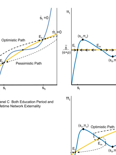
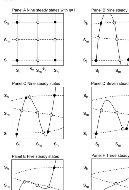
In the demarcation locus for ˙Πt, Πt is simply an increasing function of st, as denoted by a dotted
curve in Panel B of Figure 1. The demarcation locus for ˙st is represented by (st,Πt) that satisfies the
following two equations that are associated with the threshold ability level for the skill achievement:
st = 1−G(˜a)
˜
a = A(st,Πt).
The first one is denoted by the solid curve in Panel A of Figure 1 in (st,a˜) domain, which is simply a
S-shaped curve. The second one is denoted by the dotted curves for each level of Πt (iso-Π curves),
in the same panel. As Πt increases, the corresponding iso-Π curve moves down. (The curves tend to
be convex as the marginal impact of a network quality on the threshold ability level may decline asst
increases.) The combinations of (st,Πt) that satisfy the above two equations are represented by the
solid curve in Panel B of the figure, which is the demarcation locus for ˙st. Since we have achieved two
demarcation loci, we can identify steady states in this system.
s′′<1−G(A(s′′,δ¯+ρf+(αs′′))), there are at least three steady states.
Proof. See the proof in the appendix. ¥
Note that, as long as the the network externality in the skill acquisition period is strong enough
(∂A∂s
t is big enough), the dotted curves in Panel A (iso-Π curves) are tangent to the S-shaped curve
(st= 1−G(˜a) curve) at two distinct points, (su,a˜u) with Πt= Πu and (sd,˜ad) with Πt= Πd, where
Πu >Πd. In the specific case with two tangent points, the multiple steady state condition in Lemma
2 is simply satisfied when Πu >
¯
δ+f(su)
ρ+α and Πd<
¯
δ+f(sd)
ρ+α , as you can observe in Panel B of Figure 1.
Without loss of generality, we assume that there exist three steady states when the condition of
Lemma 2 is satisfied.15 When the condition is not satisfied, it is most likely that there exists a unique
steady state.16 For example, if the base salary differential ¯δ is too big or too small, the ˙Πt= 0 locus
will be placed too high or too low, and there is a unique intersection between the two loci. Whatever
the initial position s0 is, the group state will move toward the unique steady state.17 That is, if the base salary for a skilled job is much greater (smaller) than that for an unskilled job, the group skill
levelst converges to a high (low) skill steady state, regardless of the initial network quality. This is
certainly not an interesting case: the network externalities do not generate any difference in the final
economic outcome. Therefore, we will focus on the case with three steady states in this paper.
Proposition 1. Without loss of generality, there is a range of the base salary differentialδ¯∈(¯δl,¯δh),
with which there exists three distinct steady states in a homogenous group economy.
Proof. Without loss of generality, assume that the dynamic system has two distinct salary differentials ¯
δl and ¯δh, with which the ˙Πt = 0 locus is tangent to the ˙st = 0 locus in the (st,Πt) plane. Between
the two levels, there will be at least three steady states. Without loss of generality, there are three
steady states in the interval (¯δl,¯δh). ¥
Let us denote the three steady states byEl(sl,Πl),Em(sm,Πm) andEh(sh,Πh), wheresl< sm <
sh. The final economic state (s,Π) will be on either one of them. In order to examine the conversing
process to a steady state, we need a phase diagram with direction arrows (laws of motion), which are
displayed in Figure 2. The characteristics of the steady states are summarized by the following lemma.
Lemma 3. Among three steady states,El(sl,Πl),Em(sm,Πm) andEh(sh,Πh),El andEh are saddle
points andEm is a source.
15There exist more than three steady states only for very peculiar functional forms ofG,Aorf. 16It is possible that there are only two steady states, for example, when the ˙Π
t = 0 locus is tangent to the ˙st = 0
locus. We ignore this case because it can occur with a measure zero probability.
17The unique steady state is a saddle point, which is easily proven as the same way for the proof of Lemma 3. The
Proof. See the proof in Appendix. ¥
We can identify the equilibrium path (saddle path) to each saddle point,El and Eh, as described
in Figure 2. In the given example of the figure, the equilibrium paths spiral out of a source Em.
Given an initial network quality s0 ∈ (0,1), the newborn agents will calculate the expected benefits of investment Π0. Based on the calculated Π0, each agent with different innate ability (a) makes his
own skill investment decision. In their calculation of Π0, they will use the evolution rules ofstand Πt,
summarized in the formula (7). They understand that either Eh orEl should be the final economic
state. If they believe that Eh will be realized in the future, they will choose Π0 on the equilibrium path toEh. As the following generations keep the same belief, the group state will be moving along
the equilibrium path, and eventually arrive atEh. If they believe thatElwill be realized in the future,
they will choose Π0 on the equilibrium path toEl. As the following generations keep the same belief,
the group state will move towardEl along the path. Since there is no equilibrium path that converges
atEm, the newborn agents who understand the evolution rules ofst and Πt will never choose Em as
the final group state. ChoosingEh is called sharing an optimistic social consensus, while choosingEl
is called sharing a pessimistic social consensus.
Although all three steady states are mathematically unstable, two saddle points, El and Eh, are
“economically” stable in a sense that there exists a converging path to these states for any perturbation
at the states: rational economic agents who understand the dynamic system can take the saddle path
to lead the group back to the original state. However, the source Em is “economically” unstable,
because any small perturbation from the state will lead the group to move away from it: rational
economic agents will take either the optimistic path toEh or the pessimistic path toEl, because there
is no converging path toEm.
Definition 1 (Economically Stable States). A state (s′,Π′) is an economically stable state if there
exists a converging phase path to the state for any s in the neighborhood of s′. Otherwise, it is an
economically unstable state.
In the given economy with three steady states,El and Eh are economically stable states and Em
is an economically unstable state.
4.2 Overlap and Deterministic Ranges
Let the network quality eo denote the lower bound of the optimistic path to Eh, and the network
qualityep the upper bound of the pessimistic path to El. As shown in the example of Figure 2, there
exists a unique optimistic path for an initial network quality in the interval (ep,1): if the initial network
the group state (st,Πt) will move toward the high skill equilibrium (sh,Πh) by self-fulfilling investment
activities. Also, there exists a unique pessimistic path for an initial network quality in the interval
(0, eo): if the initial network quality is poor enough, there is only one reasonable social consensus about
the future, that isEl, and the group state (st,Πt) moves toward the low skill equilibrium (sl,Πl), by
the self-fulfilling investment activities. However, if the initial network quality is mediocre in (eo, ep),
there exist multiple social consensuses about the future,El and Eh, that are available to the group.
The final economic state depends on the social consensus that the newborn agents of the group choose.
If they and the following generations are optimistic, Eh will be realized in the end. If they all are
pessimistic, El will be realized in the end. Therefore, in the interval [eo, ep], the social consensus
determines the future, while the historical position determines the future outside the interval. We
denote [e0, ep] as overlap as Krugman (1991) denotes. We denote the ranges (0, ep) and (eo,1) as
deterministic ranges as the macroeconomic literature denotes.
Proposition 2. In a homogeneous group economy with two economically stable states El and Eh,
there exists a positive range of overlap, [eo, ep], with eo < ep, where the social consensus about the
future determines the final economic state among El and Eh.
Proof. See the proof in Appendix. ¥
Corollary 1. In a homogeneous group economy with two economically stable states El and Eh, the
deterministic range forEh is (ep,1), and the deterministic range forEl is(0, eo), where eo< ep.
Proof. Since there exists a unique equilibrium path outside the overlap, both ranges (ep,1) and (0, eo)
are deterministic ranges. Sinceep is the upper bound of the pessimistic path toward El, (ep,1) is a
deterministic range forEh. Sinceeo is the lower bound of the optimistic path towardEh, (0, eo) is a
deterministic range forEl. ¥
4.3 Mobilization Force and Historical Force
There are two kinds of network externalities, education period and lifetime, that affect the structure
of the economy. In order to examine the direct effect from each network externality, we compare three
distinct cases: 1) lifetime network externality only 2) education period network externality only and
3) both education and lifetime network externalities.
Lifetime Network Externality Only: the Mobilization Force
Panel A of Figure 3 describes the first case: there exists very negligible peer effects or parental
effects together with perfect provision of public schooling or no credit constraints in the skill acquisition
Panel A of Figure 1 is almost flat: ∂A(st,Πt)
∂st ≃0, or ˜a≡A(Πt),ignoring the st term. Therefore, the
˙
st= 0 locus will be like aS-shaped curve that satisfiesst= 1−G(A(Πt)). As you can observe in Panel
A of Figure 3, the overlap may to cover the whole range of network quality [0,1].18 In this case, the historical position of initial network qualitys0 does not provide any constraint in the determination of
the final economic state. The final economic state entirely depends on the social consensus, regardless
of s0. (With the bigger discounting factor ρ, the overlap may not cover the whole range of network
quality [0,1].19 Even in this case, the overlap range will be much greater than that in Panel C of Figure 3.) In other words, skill investment activities of newborn agents tend to be subject to the
“future”: the expected benefits of skill acquisition that accrues over the lifetime.
Suppose the initial network quality is s0 ∈ (sl, sh). If the group members believe that the final
state isEhinstead ofEl, the future benefits anticipated to accrue from skill acquisition Πop0 are greater
than the current level of network benefits (¯δ+f(s0)
ρ+α ), and more newborns invest in skills. The group’s
network quality improves over time and the group state converges to (sh,Πh) along the optimistic
path, as displayed in Panel A of Figure 1. If they believe that the final state is El instead of Eh,
the future benefits anticipated to accrue from skill acquisition Πpe0 is smaller than the current level of network benefits (¯δ+f(s0)
ρ+α ), and less newborns invest in skills. The group’s network quality deteriorates
and the group state converges to (sl,Πl). Therefore, the social consensus toward the future determines
the future. Group members can work together to improve the quality of the group’s social network
by sharing the optimistic social consensus, or to deteriorate the quality of the network by sharing the
pessimistic social consensus. This is what I call themobilization force of network externalities.
Education Period Network Externality Only: the Historical Force
Panel B of Figure 3 describes the opposite regime, where there is no network externality over the
course of a worker’s lifetime. The benefits of skill acquisition is just the wage differential ¯δ at each
period, and the consequent lifetime benefits are ρ+¯δα. In this case, the expectation toward the future does not play any role because the benefits of skill acquisition is fixed. The skill investment activities
of newborns are subject to the “past”: the cost level to achieve the skill. If the initial network quality
is good, the cost for the skill achievement is low. Consequently, a large fraction of newborns invest
in skill. Then, the network quality in the next period is even better because of the enhanced skill
investment rate in the previous period. Thus, even more newborns invest in skill in the next period.
18In this case, another limit set exists, which is a loop located between the optimistic path and the pessimistic path.
If economic agents believe that the network quality will fluctuate forever, the group state will be on this loop. I rule out this unique case in my study.
19Note that, the bigger ρ, the bigger ˙Π
t and the longer the vertical direction arrows in the phase diagram. As the
The network quality improves over time. If the initial network quality is poor, a small fraction of
newborns invest in skill. The next period network quality is even worse, and even less newborns invest
in skills. The network quality deteriorates over time.
The two examples are displayed in the Panel. If the initial network quality is bad, below sm, the
network quality converges to the low skill equilibriumEl. If it is good, above sm, the network quality
converges to the high skill equilibrium Eh. Therefore, the final economic state entirely depends on
the history, an initial network quality of the group. This is what I call thehistorical force of network
externalities.
Both Lifetime and Education Period Network Externalities: Two Forces Combined
Panel C of the figure display how the two forces of network externalities are interwoven in the
dynamic structure of network quality evolution. The mobilization force of lifetime network externalities
is constrained by the historical force of education period network externalities. The overlap is the
network quality range mainly governed by the mobilization force, while the deterministic ranges are
the network quality ranges mainly governed by the historical force. In the overlap, the group can be
mobilized toward the high skill steady stateEhby sharing the optimistic view together, or toward the
low skill steady stateEl by sharing the pessimistic view together. Outside the overlap, it is the initial
historical position that determines the final state. If it is high (low) enough, the group status moves
toward the high (low) skill steady state.
4.4 Size of Overlap
In the previous sections, the importance of overlap has been emphasized. Whether the initial position
is in the overlap or outside the overlap determines whether the group members can work together to
change the future by sharing optimism (or pessimism). Outside the overlap, the future is determined
through a mechanical tatonnement process. The bigger size of overlap indicates the dynamic structure
that is more governed by the mobilization force or the power of collective action. It is worthwhile
to check how the overlap size is determined, because this is an indication of the relative power of
the mobilization force and the historical force. In order to make a comparative statics analysis, let
us simplify the given model using the linear functional forms of the cost function C(a, st) and the
benefits functionf(st):
C(a, st) = ψ(a)−k1st (10)
where k1 represents the influence of education period network externality, and q1 the influence of
lifetime network externality. We further assume that the innate ability equals across the population:
a ≡ a¯. The newborn agents with the unique innate ability ¯a decide to invest when the benefits is
greater than the cost: if Πt> ψ(¯a)−k1st,xt= 1 and ˙s=α[1−st], and if Πt< ψ(¯a)−k1st,xt= 0 and
˙
s=α[0−st]. Therefore, the slanting part of the ˙s= 0 locus in Appendix Figure 1 is Πt=ψ(¯a)−k1st,
which is a demarcation line that sharply divides the evolution rule of ˙st. The demarcation locus for
Πtis Πt=
¯
δ+q0+q1st
ρ+α . In this simple system without hurting the essential structure of the economy, we
can explicitly find the optimistic and pessimistic paths and the relevant size of overlap.
Lemma 4. In the simple homogenous economy with equations (10) and (11) and the unique innate
ability level of a¯, the optimistic equilibrium path (sop,Πop) above two demarcation loci and the
pes-simistic equilibrium path(spe,Πpe) below two demarcation loci are
Πop = q1
ρ+ 2αs
op+(¯δ+q0)(ρ+ 2α) +q1α (ρ+α)(ρ+ 2α)
Πpe = q1
ρ+ 2αs
pe+δ¯+q0
ρ+α.
Proof. See the proof in Appendix. ¥
This linear equilibrium paths are described in Appendix Figure 1 with the corresponding
de-marcation loci. Using the calculated equilibrium paths and the slanting part of the ˙s = 0 locus
(Π =ψ(¯a)−k1s), we can obtain the overlap size ¯L:
L= α
(α+ρ)(1 + (k1/q1)(ρ+ 2α))
. (12)
Using the outcomes, we have the following results that have deep economic implications.
Proposition 3. In a simple economy defined in Lemma 4, the bigger the relative influence of lifetime
network externality over education period network externality (the bigger q1/k1), the larger the size
of overlap. The less the economic agents discount the future (the smaller ρ), the larger the size of
overlap.
Proof. The first derivatives of equation (12) give the results. ¥
The first result implies that, when the lifetime network externality is relatively more influential,
the mobilization force of network externalities is stronger compared to their historical force; collective
action facilitated by the formation of social consensus can play a bigger role in the determination of
the final economic state. The lower discounting factor means the greater forward-looking decision
the determination of the final outcome. This fact is reflected in the second result of the proposition.
5
Heterogeneous Group Economy
Now we come back to the two group economy summarized in the four variable dynamic system of
Theorem 1. We assume that the conditions in Lemmas 2 and 3 are applied to this economy, so that
there exist three steady states at skill levelssl,sm and sh in the fully integrated economy, or in each
group’s economy with social interactions fully separated between two groups. Note that there will
be no group disparity in the long run if there exists a unique steady state: whatever the initial skill
composition (s1
0, s20) is, the economy state (s1t, s2t) converges to the unique steady state as time goes
by. Therefore, there will no issue for the persistent group disparity through the channel of network
externalities in this case, and this is certainly not an interest in this study.
5.1 Heterogeneous Economy with Total Segregation
Let us start with the simplest case of the two group economy: fully separated social interactions
between two groups (η = 1), which can help us to have an intuition about the four dimension dynamic
structure of two group economy. The structure of this special case can be directly inferred from the
properties of the homogeneous economy because there are no interactions between the two. Using the
same definition of economically stable states in the homogeneous economy (Definition 1), a steady
state (s1′, s2′,Π1′,Π2′) is called an economically stable state if there exists a converging phase path
to the state in the neighborhood of (s1′, s2′). Obviously, there are nine steady states in this economy:
Qij(si, sj,Πi,Πj) fori∈ {l, m, h}and j∈ {l, m, h}. Among them, the following four are economically
stable states: Qll(sl, sl,Πl,Πl), Qlh(sl, sh,Πl,Πh) Qhl(sh, sl,Πh,Πl) and Qhh(sh, sh,Πh,Πh). Those
are depicted with dark circles in (s1, s2) domain in Figure 4. The other five economically unstable states are depicted with gray circles in the domain. Two separated dynamic structures are displayed
beside the domain in the figure. In an economically unstable state, any arbitrary shock to the position
may lead the economic state (s1
t, s2t,Π1t,Π2t) to move away from it, while the economic state can come
back to the original steady state after any small shock in an economically stable state.
Since there are four economically stable states, a society with an initial skill composition (s1 0, s20) will move to either of them in the long run. Once a social consensus about the future is constructed in
the society, the economic state (s1
t, s2t,Π1t,Π2t) will move to the future state of social consensus following
a unique converging path to the state. Let us check available social consensuses and corresponding
equilibrium paths for each initial skill composition (s1
5.1.1 Stable Manifolds and Manifold Ranges
First, regardless of the position ofs2
0, group 1 with an initial skill levels10 can move toward either the skill levelsl orsh following the same rule in the homogeneous economy. The optimistic path tosh is
available to the group with an initial skill positions1
0 ∈[eo,1] and the pessimistic path is available to
the group with an initial skill positions20∈[0, ep]. Those available equilibrium paths are described in
Panel A of Figure 5: the available optimistic path in pink and the pessimistic path in blue. In the
interval (eo, ep), which is an overlap, both optimistic and pessimistic paths are available. The same is
true for group 2, as displayed in Panel B of the figure.
Therefore, when boths10ands20are greater or equal toeo, the equilibrium path toQhh(sh, sh,Πh,Πh)
is available to the society. The unique converging path toQhhis a combination of two optimistic
equi-librium paths, (s1t,Π1t)opfor group 1 and (s2t,Π2t)opfor group 2. In the same way, the equilibrium path
toQll(sl, sl,Πl,Πl) is available when boths10 ands20 are smaller or equal toep. The unique converging
path toQll is the combination of two pessimistic paths, (s1t,Π1t)pe and (s2t,Π2t)pe. The set of initial
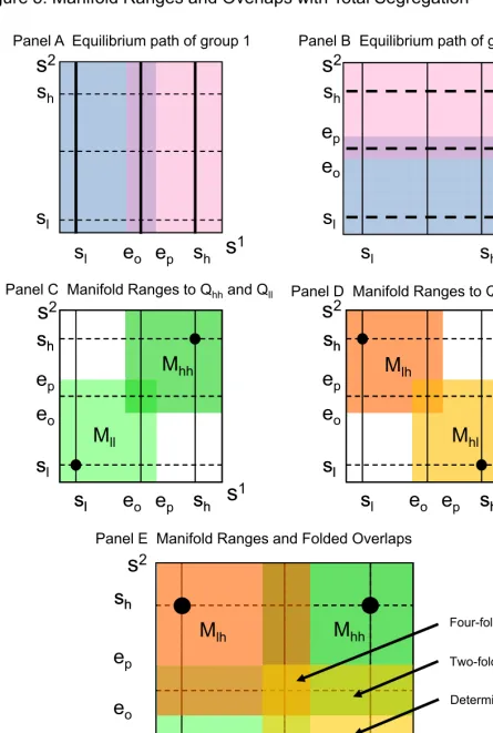
positions (s10, s20) where the converging path toQhh is available is called Manifold Range forQhh, and
colored in darker green in Panel C of Figure 3. The set of initial positions where the converging path
to Qll is available is called Manifold Range for Qll, and colored in lighter green in the same panel.
In the same way, we define the Manifold Ranges forQhl and Qlh. The manifold range for Qhl is the
set of (s10, s20)s with s1≥eo and s2 ≤ep, and is described in lighter orange in Panel D. The Manifold
Range forQlh is the set of (s10, s20)s withs1≤ep ands2 ≥eo, and is described in darker orange in the
panel.
In geometry, a collection of points on all converging paths to a limit set Q is defined as a stable
manifold to the limit set Q.20 Using the concept, we define the stable manifold to an economically stable stateQij.
Definition 2 (Stable Manifold SMij). Stable manifold SMij is a collection of (s01, s20,Π10,Π20)s that
converge to an economically stable state Qij in the dynamic system defined in Theorem 1:
SMij ≡ {(s10, s20,Π10,Π20)∈R4|(s1t, s2t,Π1t,Π2t)|(s1
0,s20,Π10,Π20) →Qij}.
The manifold range to Qij is redefined using the concept of stable manifold, which is just a
projection of the stable manifold toQij to the (s1, s2) plane.
20A limit set in geometry is the state a dynamic system reaches after an infinite amount of time has passed, by either
Definition 3 (Manifold Range Mij). Manifold rangeMij is a collection of(s10, s20)s inSMij:
Mij ≡ {(s10, s02)∈[0,1]2|(s1t, s2t,Π1t,Π2t)|(s1
0,s20,Π10,Π20)→Qij}.
5.1.2 Folded Overlaps and Deterministic Ranges
All manifold ranges are put together in Panel E of Figure 5. There are nine distinct areas: all manifold
ranges are folded in the center square, two manifold ranges are folded in the rectangles surrounding
the center square, and a unique manifold range exists in each of the corner. In the center square,
where four manifold ranges are folded, four social consensuses about the future are available to the
members in the society: the consensus ofQhh, that ofQlh, that ofQhl and that ofQll. Depending on
the constructed social consensus, the economic state will move toward one of four economically stable
states along a unique converging path. The social consensus is a combination of the expectation to
group 1’s final state and that of group 2’s final state, as summarized in the following table.
Group 2 \ Group 1 Pessimistic Expectation Optimistic Expectation
Optimistic Expectation Qlh Qhh
Pessimistic Expectation Qll Qhl
If the initial skill composition (s10, s20) is in one of four rectangles, where two social consensuses are available, the expectation to one group’s final state is critical in the determination of the social
consensus about the future. For example, in the rectangle placed in the top middle, two manifold ranges
are folded, Mlh and Mhh, and two social consensus about the future are available: the consensus of
Qlh and that of Qhh. Group 2 will move toward sh regardless of social consensus, because only the
optimistic equilibrium path is available to the group: s2t → sh. Group 1’s expectation toward the
future is important in the determination of social consensus and in the consequent equilibrium path.
If group 1 holds an optimistic expectation toward the future, the economic state (s1t, s2t,Π1t,Π2t) will
converge toQhh. Otherwise, it will converge toQlh.
If an initial skill composition (s10, s20) is in one of four corner areas, the economic state will converge to the unique economically stable state (Qij) in the area. Social consensus about the future is fixed as
Qij among the rational economic agents. Thus, the expectation toward the future does not play any
critical role in the determination of the final state, but the location of the initial skill composition, so
calledhistory, determines the final state. To clarify the distinct areas determined by manifold ranges,
I define a folded overlap where multiple manifold ranges are folded, and a deterministic range which
is covered by a unique manifold range.