On the Numerical Solutions of One and Two Stage Model of Carcinogenesis Mutations with Time Delay and Diffusion

On the Numerical Solutions of One and Two-Stage Model

of Carcinogenesis Mutations with Time Delay and

Diffusion

*

Ishtiaq Ali

Department of Mathematics, COMSATS Institute of Information Technology, Islamabad, Pakistan Email: [email protected]

Received August 15, 2013; revised September 15, 2013; accepted September 23, 2013

Copyright © 2013 Ishtiaq Ali. This is an open access article distributed under the Creative Commons Attribution License, which permits unrestricted use, distribution, and reproduction in any medium, provided the original work is properly cited.

ABSTRACT

In this paper, we focused on numerical solutions of carcinogenesis mutations models that are based on reaction-dif- fusion systems and Lotka-Volterra food chains. We consider the case with one and two-stages of mutations with appro- priate initial conditions and the zero-flux boundary conditions. The main purpose is to construct a stable discretization scheme, which allows much accuracy than those of a standard approach. To this end, we use the spectral method to postprocess numerical solutions for the proposed model by using some classical methods for solving differential equa- tions. The implementation of the algorithm is simple and it does not need to solve the linear or nonlinear system (in case the model is nonlinear). We simulate the one and two-stage carcinogenesis mutations model and compared the results with previously published ones.

Keywords: Carcinogenesis Mutations; Delay and Diffusion; Spectral Postprocessing; Numerical Simulations

1. Introduction

The struggle for finding an effective and permanent cure for tumor continues to challenge scientists has been made by a lot of progresses in discovering new methodologies which are helpful in successful treatments to reduce and even clear tumors. Mathematical modeling is one of the tools to improve the cancer therapy. Carcinogenesis is a very complicated process and one need a comprehensive study to fully understand it. Tumors are derived from one or more normal cells that have undergone malignant transformation. The immune response to tumors depends on how antigenic the tumor is. A cell that has undergone significant mutation results in a tumor is easier to be recognized as foreign (i.e. more antigenic) than one that

differs only slightly from a healthy cell [1]. For different types of cancers, it is possible to divide the process into different number of stages, normally between 4 and 7 stages, which depends on the type of tumor [2].

In this paper, we study a simple model of carcinogene- sis mutations of DNA, which originally comes from [3]

and was also studied in [4-9], which describe a process of carcinogenesis mutations with n different steps of muta-

tions (from normal to malignant cells). The model is ex- pressed in terms of system of partial differential equation, in which the latest stage of mutation has different forms depending on whether it has growth advantage in favor- able or competitive conditions or disadvantage of growth in unfavorable and competitive conditions. For simplicity in this paper, we only consider the latest stage in unfa- vorable conditions, as in the case of favorable conditions there is no possibility to cure the disease without any treatment. For more details we refer to [10,11].

The current work provides the computational and im- plementational details needed to study the dynamics of these equations [12]. A detailed analysis of the one-stage model equations was undertaken in [4]. We use spectral methods to postprocess numerical solutions, which use the numerical solutions of a lower order method to serve as starting value of the spectral methods. The iteration uses the Gauss-Seidel type strategy, which can be very useful in terms of improving the accuracy of the numeri- cal solutions. In particular for the problems in which ac- curacy is the only issue and some conservatives proper- ties are even more important for large time simulation. Also there is no need to solve a linear or nonlinear sys- *_{Numerical solutions of one and two-stage model.}

tem of equations as we do need in case of using some other numerical methods [13].

The paper is organized as follows. Section 2 and 3 is used for the description of models in detail. In Section 4 and 5 we describe in detail the spectral postprocessing approximation for the proposed models. Section 6 is used for the numerical simulations and discussions, followed by the concluding remarks in Section 7.

2. Formulation of the Model

Let us consider Yj as a density of mutant cells of the j-th

stage at position

 

t x, where j0,1, 2,3, , . n To

develop a multistage model for mutant cells densities at stage Yj, j0,1, 2,3, , , n where Y0 will be the ini- tial stage, Yj



j1, 2,3, , n1



the density of interme-

diate stages, and Yn represents the density of the final

stage. The system of equations for the density function is given by [2].

1 1 1

1 .

j j

j j i j j j j j j j

j

Y Y

D Y a Y Y Y Y Y

t K    

 



   _  _ 

 _{ } (1)

The final stage of mutation occurs when cancer cells become malignant and metastasize. We assume that for the malignant mutation in the final stage, the carrying capacity is unlimited; that is Kn , thus Equation (1)

becomes

1,

n

n n n n n n n Y

D Y a Y Y Y

t  



   

 (2)

3. Formulation of One and Two-Stage

Mutation

The full blown developed malignant mutation can be described in the following system of the n-stage model,

that is initial, benign, and malignant,

0 0

0 0 0 0 1 0 1

0

1 1 1

1

1 ,

1 ,

,

j j

j j i j j j j j j j j

n

n n n n n n n

Y Y

D Y a Y Y Y

t K

Y Y

D Y a Y Y Y Y Y

t K

Y

D Y a Y Y Y t                   _{ }       _  _   _{ }       (3)

After rescaling Equation (3) it can be written in the following simplified form

 

 





 



 



 

 

 









 

0

0 0 1

0 0

1

1 0 1

1 1

, , 1 , ,

, ,

, , ,

, , ,

y

t x y t x a y t x y t x t

d y t x y

t x y t x y t x y t

t x d y t x

                     (4)

where y0 represents the density of normal cells at time ,

t and position x, y₁ stands for malignant cells, con-

stant

0 1 1 0 1

0 1

1 1 1 1

, , , ,

a d D

a d d

a a a d a

   

    

are positive, delay 1

s

a



  is non-negative and

 

0, ,

x  with the Neumann boundary and initial con-

ditions

 

 

0,

 





 

, 0, 0,1,

, , 0, ,0 , 0, , 0,1.

i x

i i

y

t x i

t

y t x  t x t  x i

 



  

      

It is reasonable to consider interaction not only be- tween cells on subsequent stages of mutations, and there- fore we consider the following two-stage model

 

 





 



 

 



 

 

 





 



 





 



 

 

 



 



   

 

0

0 0 0 1 1

1 2 0 0

1

1 1 1 2 2

1 0 1 1 1 1

2

2 2 1 2 1 2

2 0 2 2 2

, , 1 , ,

, , ,

, , 1 , ,

, , , ,

, , , ,

, , , ,

y

t x y t x a y t x y t x t

y t x d y t x y

t x y t x a y t x y t x t

y t x y t x d y t x y

t x y t x y t x y t x t

y t x y t x d y t x

                                      (5) subject to

 

 

 





 

0,

, 0, 0,1, 2

, , 0, ,0 , 0, , 0,1, 2.

i x

i i

y

t x i

t

y t x  t x t  x i

 



  

      

4. Spectral Postprocessing Technique

In this section, we will describe in detail the spectral methods for Equations (4) and (5). We first use a finite difference scheme in time and spectral methods in space.

4.1. Finite Difference Scheme

Let



1



,

2

j j

s

x    tn n t with

 

₀

M j _j

s

 are

are Legendre-Gauss-Lobatto points in



1,1



and

.

T t

N

  Without losing any generality, we can choose

N such that   k t, where k is an integer. Denote

by









1

1, 1 1 1 1 0, 1

T T

1 1,0 1, 0 0,0 0,

, , , ,

, , , , , ,

n n

j n j j n j

n n n n n n

M M

y y t x y y t x

y y y y y y



    

   

then the implicit difference scheme is given by enforc- ing Equation (4) at



tn1,xj



1

1, 1, 1 1

1, 1 2 1

1 1

0, 1, for 1 1,

n n

j j n n

j n k n k

j j

y y

y d D y t

y y j M

                 (6) where 2 2 2

D   D_



  with D is the differential ma trix associated with Legendre-Gauss-Lobatto nodes, see [13] for details. Rearranging Equation (6) in terms of matrix form, we have









1 1 1

1 2 1 1 0 1

1 n n n k n k

n

t I d D y  y ty   y  

       (7)

where  means element-wise multiplication of two vectors. Here we should remark, considering the bound- ary conditions in Equation (4), that is the first and the last equation in the above equation, that is Equation (7) do not hold any more. Instead, we must replace those two equations by directly discretizing the boundary condi- tions respectively. Similarly the semi-implicit scheme for

1 0,nj

y  is given by





1







1



1 2 0n 0n 0n 1 0n 1n ,

I td D y y  ty  a y y  (8)

where we utilize the updated 1 1

n

y  in Equation (7). More-

over, to replace the first and the last equations in Equa- tion (8), we also need to enforce the boundary conditions of y0 that

1 1

0,: 1n 0 and M,: 1n 0.

D y   D y  

Applying the same implicit and semi-implicit finite difference scheme to the two-stage mutation model, we have the following system

































2 2 1 1 1

2 2 2

1 1

2 2 1 2 2 0 2

1

1 2 1

1

1 1 1 1 2 2

1 1

1 0 1

1

0 2 0

1 1

0 0 0 0 1 1 1 2

,

1

,

1

n n k n k

n n n

n

n n n n

n k n k n

n n n n n

I t I td D y

y t y y t y y

I td D y

y ty a y y

t y y

I td D y

y ty a y y y

                                                  (9)

where i

i

k t





 are assumed to be integer for simplicity.

In fact, we can deal with any i by interpolation if there

is no suitable t such that k_i be integers. Moreover,

to satisfy the boundary conditions which is similar to

one-stage mutation model, we can replace the first and the last equations in each matrix form by

1 1

0,: 1 0 and ,: 1 0,

n n

M

D y  D y  

for i0,1, 2, respectively.

5. Postprocessing

It is well known that backward Euler finite difference scheme in time direction is of the first order accuracy, which is much worse than the spectral accuracy in spatial direction. Therefore, to achieve the balance between the errors in two directions, we use spectral postprocessing in [13] to enhance the accuracy in time direction based upon the backward Euler finite difference scheme.

To describe the time marching scheme clearly, we give some notations as follows. Split the time interval

 

0,T

into several subintervals, i.e.,

 

0,T Uitp_i,tp_i₁, for

simplicity we can take tp_i₁tp_i. Let



1



2

i

ij tp sj



    with sj given above as Legendre-

Gauss-Lobatto points in



1,1



.

Integrating Equation (4) from tp_i to ik, we get

 

 



 



 

1 1 0 1 2

1 2 1

, d , d

, , d

, d

ik ik

pi pi

ik pi ik pi t t j j t t

y x y x

t

y x y x

d y x x                  _{ }       









(10)

using the



N1



-point Legendre Gauss-Lobatto quad-

rature formula relative to the Legendre weights on the right hand side of Equation (10) gives















 











1 1 0 1 0

1 1 1

0

, , 1

4

, ,

, 2 , ,

i

ik j p j k

M

ikm j ikm j

m

M

ikm j jk ikm k m n

y x y t x s

y x y x

y x d D y x

                   





(11)

where



1



1



.

4

i

ikm tp sk sm



     In the above for-

mula, to explicitly update y1



ik,xj



, we need to evalu-

ate y1



ikm,xj



by some approximations. Fortunately,

we have the Euler scheme solution (7) as an initial ap- proximation and then interpolation to the Legendre- Gauss-Lobatto points in tp_i,tp_i₁. Denote by





1 ,

n ik j

y  x the n-th loop of post-processing solution,

whereas for n0, it is the linear interpolation of the

is given by











































 











1 1 2 1 1, 0 0 1

1 1, 1 1,

0 1 1 1 1 1 0 0 1 1

, , 1

4 , , , , 2 , , , i n

ik j p j k

M M

N

i e j e ikm

m e

k

N n

i e j i e j e ikm

e

M n

ie j e ikm e k

M k

n

jk ie k e ikm

k e

M n

ie j e ikm m e k

y x y t x s

y x F

y x y x F

y x F

d D y x F

y x F

                                    _  _     _{ }    _    _    _ 

 











(12)

where Fe

 

 is the e-th Lagrangian interpolation poly- nomials associated with Legendre-Gauss-Lobatto points. Here we remark that in Equation (12) the updated infor- mation of ₁n



,



ik j

y  x is immediately used to obtain





1 i k, 1, j

y  _ x . Similarly, we can get the spectral post

processing scheme for y₀ in Equation (4):

























0 0

0, , 0, , 0, ,

0

0 1

0

, , 1

4

1

2 ,

i

n n

ik j p j k

M

temp j temp j temp j m

M

jk ikm k m n

y x y t x s

y a y y

d D y x

             





(13) where

































1

0, , 0

0

1 0

1, , 1

0 1 1 1 , , and , , k n

temp j ie j e ikm e

M n

ie j e ikm e k

k n

temp j ie j e ikm e

M n

ie j e ikm e k

y y x F

y x F

y y x F

y x F

                   









For the sake of compactness, we shall not give the full spectral post processing scheme for the two stage Equa- tion (5) here. However, the idea is same as the one stage model. Instead, we give an algorithm to implement the spectral post processing scheme in detail.

Algorithm 5.1 (Spectral Post-Processing)

1) Initialize 0





0





1 0,0, j and 0 0,0, j

y  x y  x by interpo-

lation from Equations (7) and (8) 2) For i1 to # of subintervals

3) For n0 to # of loops on post processing

4) For k0 to M

5)



1



,



1



1



2 4

i i

ik tp sk ikm tp sk sm

 

        

6) Compute y₁



ik,xj



by Equation (12)

7) Compute y₀



ik,xj



by Equation (13)

8) End k

9) End n

10) End i

6. Numerical Simulation and Discussion

In the following, some numerical simulations were car- ried out. In our computations we use the Legendre-Gauss quadrature with weights



₂



 

2

1

1 _{, 0 .}

1

j

j N j

j N

x L x





    

 _{ }

In case of one-stage model the initial functions

 





 

0 t x, 0.2 0.1cos 4 x , ,1 t x 1.77

      for healthy

and cancer cells respectively and the parameters value

6 6

0 1

2, 1e , 4e , 0.9, 5.

a d   d     (14)

and for the two-stage model, we use

6 6

0 1 0 1

6

2 1 2 1

2 1 2

2, 1, 1e , 4e ,

4e , 0.5, 0.25, 2,

3, 0.1, 0.2.

a a d d

d   

                 (15) with

 





 

 

0 1 2

, 0.2 0.1cos 4 , , 1.77

, 1.77

t x x t x

t x

 



   



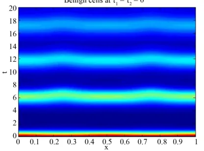
We start our simulation for the one-stage model, which is system of Equation (4) with small delay in which the steady state is positive; we observe the oscillatory be- havior of the system with different mode of frequencies. The oscillation is then smooth because of the steady state (Figures 1 and 2). Increasing the delay term and fixing

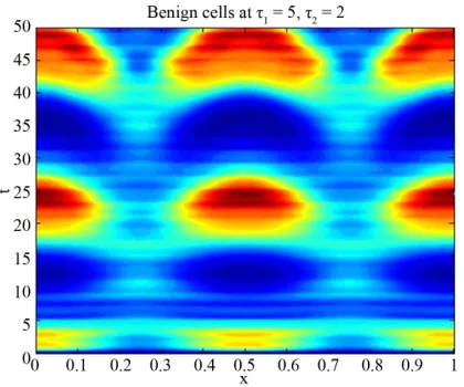
the other parameters, one can observe a very strong os- cillatory behavior of the system. For a very large value of delay term, the solution behaves like traveling waves (Figures 3 and 4). As the dynamics of the system is pe-

riod, it suggests that traveling wave solutions appear for the system with delay and diffusion. The same was ob- served for the two-stage model, which is system Equa- tion (5) (Figures 5-10). In conclusion, we can say that

[image:5.595.68.278.84.259.2] [image:5.595.313.532.85.270.2]

Figure 1. Simulated solution of system (4) for  0.1, using the parameters values of Equation (14).

Figure 2. Simulated solution of system (4) for  0.1, using the parameters values of Equation (14).

[image:5.595.66.280.305.481.2]

Figure 3. Simulated solution of system (4) for  5, using the parameters values of Equation (14).

[image:5.595.309.535.314.503.2]

Figure 4. Simulated solution of system (4) for 5, using the parameters values of Equation (14).

Figure 5. Simulated solution of system (5) for 120,

using the parameters values of Equation (15).

[image:5.595.68.278.521.702.2] [image:5.595.321.529.550.704.2]

[image:6.595.316.531.85.268.2]

Figure 7. Simulated solution of system (5) for ₁₂0, using the parameters values of Equation (15).

Figure 8. Simulated solution of system (5) for 15,22,

[image:6.595.68.280.85.265.2]

using the parameters value of Equation (15).

Figure 9. Simulated solution of system (5) for 15,22,

[image:6.595.69.278.310.485.2]

using the parameters value of Equation (15).

Figure 10. Simulated solution of system (5) for ₁5,

2 2

  using the parameters value of Equation (15).

7.

Concluding Remarks

It has been the aim of this paper to use a spectral post- processing technique for the numerical solutions of one and two-stage model of carcinogenesis mutations with time delay and diffusion. The spectral postprocessing with the coarse-mesh symplectic initial guess produces high accurate approximate solution. It also saves a sig- nificant amount of computational time over the standard schemes. We compared the results obtained by simulate- ing the one and two-stage model with the available one and find it with good agreement. The future work in- cludes the theoretical stability analysis of the proposed method and its extension to higher dimensions.

8. Acknowledgements

The author is very grateful to Professor Urszula Forys of the Institute of Applied Mathematics and Mechanics Fa- culty of Mathematics, Informatics and Mechanics Uni- versity of Warsaw, Poland for her many discussions and Xu Xiang of MSU for his help in Algorithm.

REFERENCES

[1] J. C. Arciero, T. L. Jackson and D. E. Kirschner, “A Mathematical Model of Tumor-Immune Evasion and siRNA Treatment,” Discrete and Continuous Dynamical Systems, Series B, Vol. 4, No. 1, 2004, pp. 39-58. [2] S. Kruś, “Pathological Anathomy,” PZWL, Warsaw, 2001. [3] R. Ahangar and X. B. Lin, “Multistage Evolutionary Mo-

del for Carcinogenesis Mutations,” Electronic Journal of Differential Equations, Conference 10, 2003, pp. 33-53.

[image:6.595.69.279.530.705.2]

[5] U. Foryś, “Biological Delay Systems and the Mikhailov Criterion of Stability,” Journal of Biological Systems, Vol.

12, No. 1, 2004, pp. 45-60.

[6] U. Foryś, “Stability Analysis and Comparison of the Models for Carcinogenesis Mutations in the Case of Two- Stages of Mutations,” Journal of Applied Analysis, Vol.

11, No. 2, 2005, pp. 200-281.

[7] U. Foryś, “Multi-Dimensional Lotka-Volterra System for Carcinogenesis Mutations,” Mathematical Methods in the Applied Sciences, Vol. 32, No. 17, 2009, pp. 2287-2308.

[8] U. Foryś, “Comparison of the Models for Carcinogenesis Mutations—One-Stage Case,” The Proceeding of the 5th National Conference on Mathematics, Applied to Biology and Medicine, Święty Krzyż, 2004.

[9] J. D. Murry, “Mathematical Biology 1: An Introduction,” Springer, Berlin, 2002.

[10] J. D. Murry, “Mathematical Biology 11: Special Models and Biochemical Applications, Interdisciplinary Applied Mathematics,” Springer, Berlin, 2003.

[11] J. D. Murry, “Mathematical Biology 11: Special Models and Biochemical Applications, Interdisciplinary Applied Mathematics,” Springer, Berlin, 2003.

[12] M. R. Garvie, “Finite-Difference Schemes for Reaction- Diffusion Equations Modeling Redator-Prey Interactions in MATLAB,” Bulletin of Mathematical Biology, Vol. 69,

No. 3, 2007, pp. 931-956.

[13] T. Tang and X. Xu, “Accuracy Enhancement Using Spec- tral Postprocessing for Differential Equations and Integral Equations,” Communications in Computational Physics,