Alpha root Processes for Derivatives pricing

Munich Personal RePEc Archive

Alpha-root Processes for Derivatives

pricing

Balakrishna, B S

11 January 2010

Online at

https://mpra.ub.uni-muenchen.de/21396/

Alpha-Root Processes for Derivatives Pricing

B. S. BALAKRISHNA

January 11, 2010, Revised: February 16, 2010.

Abstract

A class of mean reverting positive stochastic processes driven by 𝛼−stable

distri-butions, referred to here as 𝛼−root processes in analogy to the square root process

(Cox-Ingersoll-Ross process), is a subclass of affine processes, in particular continuous state branching processes with immigration (CBI processes). Being affine, they provide semi-analytical results for the implied term structures as well as for the characteristic exponents for their associated distributions. Their use has not been appreciated in the field perhaps due to lack of an efficient numerical algorithm to supplement their semi-analytical results. The present article introduces a convenient formulation of such processes, CBI processes in general, in the form of pure-jump processes of infinite activ-ity. The formulation admits an efficient simulation algorithm that enables an extensive investigation of their properties.

Stochastic processes are the building blocks of modeling discipline. Though Brownian motion has been largely successful in this regard, there are certain areas where more advanced processes could be helpful. This is especially so in mathematical finance wherein alternate processes have been utilized, in particular to provide an explanation to parameter smiles, such as volatility smiles or correlation smiles. Among other approaches, a class of stochastic processes called 𝛼₋stable L´evy processes have been used for this purpose with encouraging results. Because applicable𝛼usually lies between 1 and 2, and the associated stable processes can have negative values, their use has been largely limited to their exponentials as stochastic variables of interest. This makes them analytically intractable for many objects of interest, such as term structures of discount factors in interest rate modeling or survival probabilities in credit risk modeling.

It is known that the Cox-Ingersoll-Ross process, also known as the square-root process, though confined only to the positive real axis, admits analytical results for term structure modeling. It belongs to a class of affine processes, the spot rate in interest rate modeling being related affinely to the short rate. It is driven by Brownian motion which in the language of stable processes has 𝛼 = 2. A natural question then arises as to whether there exist

𝛼₋root processes driven by 𝛼₋stable distributions, and whether they too exhibit the affine property. As it turns out, the answer to this question is pleasantly in the affirmative. 𝛼₋root processes thus provide a natural and appealing approach to affine jump diffusion processes

by incorporating jumps into the diffusion component itself to turn it into an𝛼₋root process, rather than extending the process to include a jump component.

The class of affine processes is a well-studied branch of mathematics, and has been char-acterized in generality by Duffie, Filipovic and Schachermayer [2003]. However, this class being rather large, identification of specific affine processes for their usefulness is important in itself. Being a subclass of affine processes, in particular continuous state branching pro-cesses with immigration (CBI propro-cesses), and a natural extension of the square-root process,

𝛼₋root processes have caught the attention of researchers in the field. For instance, they are briefly touched upon by Carr and Wu [2004] as an activity process for generating random time. Their use has not been appreciated in the field perhaps due to lack of an efficient nu-merical algorithm to supplement their semi-analytical results. The present article introduces a convenient formulation of such processes, CBI processes in general, in the form of pure-jump processes of infinite activity. The formulation admits an efficient simulation algorithm that enables an extensive investigation of their properties. The algorithm is also adaptable to the case of standard mean reverting processes (Ornstein-Uhlenbeck-Type processes) driven by𝛼₋stable processes, or L´evy processes of infinite activity.

Section 1 introduces the 𝛼₋root process, CBI process in general, in the form of a mean-reverting pure-jump process of infinite activity and presents semi-analytical solutions for the implied term structures and the Laplace exponents. Section 2 presents closed form expressions for the Laplace exponents in some special cases. Section 3 presents an efficient Monte Carlo simulation algorithm that enables a numerical investigation of the process. Section 4 discusses the simulation results. Semi-analytical solutions are derived in Appendix A. The results of a numerical investigation are presented in Figures 1-10.

1

Alpha-Root Process

Let us start with the following pure jump process for a positive stochastic variable 𝑟(𝑡),

𝑑𝑟(𝑡) = [𝜙(𝑡)₋𝑚𝑟(𝑡)]𝑑𝑡+

∫ ∞

𝑧=0

ℎ(𝑧/𝑟(𝑡))𝑑𝑀(𝑑𝑧, 𝑡). (1)

Here𝑑𝑀(𝑑𝑧, 𝑡) = 𝑑𝑁(𝑑𝑧, 𝑡)₋𝑑𝑧𝑑𝑡where𝑁(𝑑𝑧, 𝑡)s are independent Poisson processes. Pro-cess𝑁(𝑑𝑧, 𝑡) is of intensity𝑑𝑧 and is associated with the interval (𝑧, 𝑧+𝑑𝑧). If𝑁(𝑑𝑧, 𝑡) jumps up by one at time 𝑡, 𝑑𝑁(𝑑𝑧, 𝑡) causes 𝑟(𝑡) to jump up by ℎ(𝑧/𝑟(𝑡−)) where 𝑡− is just prior

to 𝑡. We may refer to ℎ(𝑥) as the jump function. It is taken to be nonnegative, integrable from 𝑥 = 0, going to zero as its argument 𝑥 _{→ ∞}. 𝑀(𝑑𝑧, 𝑡) is the compensated Poisson process (a Martingale). Parameter 𝑚 is the mean reversion rate. Drift 𝜙(𝑡) is assumed to be positive. Note that the total intensity of the Poisson processes is infinite and hence the stochastic process is of infinite activity (however, effective intensity depends on the jump function and is not necessarily infinite).

An attractive feature of the above process is that it is an affine model, just as the well-known square-root process is. Note that process (1) is written in somewhat an unconventional way. It is usual to regard jump ℎ as an independent variable with the Poisson intensity

process, in particular a CBI process (for constant 𝜙(𝑡), that could also have square-root diffusion and 𝑟₋independent nonnegative jump component), in the form of a stochastic differential equation that forms the basis of a simulation to be discussed later.

Being an affine model, process (1) admits semi-analytical results for the implied term structures as well as for the characteristic exponents for their associated distributions. The following result is derived in Appendix A,

E𝑡 { exp [ − ∫ 𝑇 𝑡

𝑑𝑠𝑢(𝑇 ₋𝑠)𝑟(𝑠)

]} = exp [ − ∫ 𝑇 𝑡

𝑑𝑠𝜙(𝑠)𝐵(𝑇 ₋𝑠)₋𝐵(𝑇 ₋𝑡)𝑟(𝑡)

]

, (2)

where 𝑢(𝜏) is some deterministic function and 𝐵(𝜏), satisfying𝐵(0) = 0, is a solution of

𝑑𝐵(𝜏)

𝑑𝜏 +𝑚𝐵(𝜏) = 𝑢(𝜏) +

∫ ∞

0

𝑑𝑥_{1₋ℎ(𝑥)𝐵(𝜏)₋exp [₋ℎ(𝑥)𝐵(𝜏)]_}. (3)

Result (2) features the affine property, the expression within square brackets being related affinely to𝑟(𝑡). For term structure modeling, one is interested in solving the above equation with 𝑢(𝜏) = 1. If interested in the Laplace transform E𝑡{exp [−𝑢𝑟(𝑇)]} of the probability

density function of 𝑟(𝑇), or its negative logarithm known as the Laplace exponent, the equation is solved in the absence of 𝑢(𝜏), but under the initial condition𝐵(0) =𝑢.

The above result is for a general jump function ℎ(𝑥). For ℎ(𝑥) = 𝑎𝑥−1/𝛼

, 1 < 𝛼 < 2, we have ℎ(𝑧/𝑟)_∝𝑟1/𝛼 _{and (1) may be referred to as an𝛼−root process. Equation for𝐵(𝜏)}

then becomes

𝑑𝐵(𝜏)

𝑑𝜏 +𝑚𝐵(𝜏) = 𝑢(𝜏)−𝜎

𝛼_[𝐵(𝜏)]𝛼

, 1< 𝛼 <2,

= 𝑢(𝜏)₋𝜎𝐵(𝜏) ln𝐵(𝜏), 𝛼= 1. (4)

where 𝜎 is 𝑎[𝛼Γ(₋𝛼)]1/𝛼 for 1 < 𝛼 < 2 and is 𝑎 for 𝛼 = 1. Equation for 𝛼 = 1 is also presented above, though it needs to be treated as a special case. For the Laplace exponent, the above can be solved with 𝑢(𝜏) = 0 and 𝐵(0) =𝑢 to obtain

𝐵(𝜏) = 𝑒−𝑚𝜏

{

𝑢−(𝛼−1)

+𝜎

𝛼

𝑚

[

1₋𝑒−(𝛼−1)𝑚𝜏]

}−1/(𝛼−1)

, 1< 𝛼 <2,

= exp[𝑒−𝜎𝜏(

ln𝑢+ 𝑚

𝜎

)

−𝑚_𝜎], 𝛼 = 1. (5)

Case 𝛼 <1 turns out to be inconsistent. These results have a limit as 𝛼_→2 (given a fixed

𝜎) to correspond to the case of the square-root process. Closed form expressions for the Laplace exponent can be obtained in some special cases as discussed in the next section.

Drift 𝜙(𝑡) has been assumed to be positive. This ensures that the origin is inaccessible, that the probability density of 𝑟(𝑇) as 𝑟(𝑇) _→ 0 goes to zero. This can be examined, as usual in Laplace transforms, by looking at the 𝑢 _{→ ∞} limit of 𝑢E𝑡{exp [−𝑢𝑟(𝑇)]}. The

leading contribution comes from the integral in (2) near 𝑠=𝑇,

𝑢E𝑡{exp [−𝑢𝑟(𝑇)]} ∼𝑢exp

[

−𝜙(𝑇) 𝑢

2−𝛼

(2₋𝛼)𝜎𝛼

]

Given 𝜙(𝑡) > 0, this goes to zero as 𝑢 _{→ ∞}. For 𝛼 = 2, one obtains the well-known requirement𝜙(𝑡)> 𝜎2 _{(volatility of the square-root process is 𝜎}√_{2 in our scale convention).}

As for𝛼= 1, 𝐵(𝜏)_{→ ∞}as𝑢_{→ ∞} for all𝜏 so that the above quantity goes to zero for any

𝜙(𝑡)_≥0 (in this case, 𝜙(𝑡) can be zero).

The 𝛼₋root process can be viewed as being driven by an 𝛼₋stable L´evy process. This is analogous to the square root process being driven by the Brownian motion. To see this, consider small 𝜏 = 𝑇 ₋ 𝑡 when 𝐵(𝜏) _≃ (1₋𝑚𝜏)𝑢 ₋ 𝜎𝛼_{𝜏 𝑢}𝛼 _{and the Laplace exponent}

approximates to

[𝑟(𝑡) + (𝜙(𝑡)₋𝑚𝑟(𝑡))𝜏]𝑢₋𝜎𝛼𝑟(𝑡)𝜏 𝑢𝛼. (7)

The 𝑢𝛼 _{term is the Laplace exponent of a stable distribution of index𝛼 and skew parameter}

one (maximally skewed to the right) with zero location, the term linear in𝑢arising from the deterministic part of the𝑟₋process. Its scale parameter is𝜎(𝑟(𝑡)𝜏)1/𝛼_{(times [−cos(𝜋𝛼/2)]}1/𝛼

to be exact), as expected with the𝛼₋root of 𝑟(𝑡) attached (similar analysis can be done for

𝛼= 1). Given the above infinitesimal result, one can indeed recover the full Laplace exponent using the law of iterated expectations. Note that infinitesimally, the𝛼₋root process can be viewed as being driven by a time-scaled stable process, 𝜏 getting effectively scaled by 𝑟(𝑡). This is a stochastic scaling of time, scaling by the stochastic process 𝑟(𝑡) itself. This gives us an alternate view of process (1) for generalℎ(𝑥) as well, providing a relationship between CBI processes and L´evy processes (known as Lamperti representation).

The expression for term structure in (2) involves convolution of 𝜙(𝑠) and 𝐵(𝑠) (consider

𝑡 = 0). When modeling term structure models, say for interest rates or credit spreads, one approach is to imply the drift 𝜙(𝑡) from the given data on discount factors or survival probabilities as the case may be. If this deconvolving procedure is not convenient, one may consider the well-known approach in affine modeling of working with a constant𝜙, but with the stochastic variable 𝑟(𝑡) related to the variable of interest by a deterministic shift that is implied from the given data (see Brigo and Alfonsi (2005) for such an approach with the square root process).

2

Laplace Exponents

The Laplace exponent of the distribution of 𝑟(𝑇) can be obtained given the solution (5) for

𝐵(𝜏). For constant drift 𝜙(𝑡) =𝜙 and for 1< 𝛼 <2, this gives for the exponent

𝜈𝜙 𝑚𝑞𝜈

∫ 1+𝑝𝑢1/𝜈

1

𝑑𝑥𝑥−𝜈(

1 +𝑞𝑢1/𝜈 ₋𝑥)𝜈−1

+𝑟(𝑡)𝑒

−𝑚(𝑇−𝑡)

𝑢

(1 +𝑝𝑢1/𝜈₎𝜈 , (8)

where𝜈 = 1/(𝛼₋1), 𝑞=𝜎𝛼_{/𝑚 and 𝑝=𝑞(1−𝑒}−(𝛼−1)𝑚(𝑇−𝑡)

). The integral can be expressed in terms of incomplete beta functions. For small 𝑢, the exponent has the expansion

[

𝜙

𝑚(1−𝑠) +𝑟(𝑡)𝑠

]

𝑢₋

{

𝜙

𝑚𝛼[𝑞(1−𝑠)−𝑝𝜈𝑠] +𝑝𝜈𝑟(𝑡)𝑠

}

𝑢𝛼, (9)

where𝑠 =𝑒−𝑚(𝑇−𝑡)

stable distribution of index 𝛼). Closed form expression for the exponent can be obtained if

𝑚= 0, that reads

𝜙𝑢2−𝛼

(2₋𝛼)𝜎𝛼

[

1₋(

1 +𝑝𝑢𝛼−1)−(2−𝛼)/(𝛼−1)]

+ 𝑟(𝑡)𝑢 (1 +𝑝𝑢𝛼−1

)1/(𝛼−1), (10)

where 𝑝 = (𝛼₋1)𝜎𝛼_{(𝑇 −𝑡). If 𝑚 ∕= 0, closed form expressions can be obtained for some}

special values of𝛼. For the limiting case of 𝛼= 2, we obtain the well-known result

𝜙

𝜎2ln(1 +𝑝𝑢) +

𝑟(𝑡)𝑒−𝑚(𝑇−𝑡)

𝑢

1 +𝑝𝑢 , (11)

where 𝑝 = (𝜎2_{/𝑚)(1−𝑒}−𝑚(𝑇−𝑡)

). This is the exponent of the non-central chi-square distri-bution (volatility of the square-root process is𝜎√2). For 𝛼= 3/2, one obtains

2𝜙 𝑚𝑞2

{

𝑝√𝑢(1 +𝑞√𝑢) 1 +𝑝√𝑢 −ln

(

1 +𝑝√𝑢) }

+𝑟(𝑡)𝑒

−𝑚(𝑇−𝑡)

𝑢

(1 +𝑝√𝑢)2 , (12)

where 𝑞=𝜎3/2_{/𝑚 and 𝑝=𝑞(1−𝑒}−𝑚(𝑇−𝑡)/2

). For 𝛼= 4/3, the exponent is

3𝜙 𝑚𝑞3

{

𝑝𝑢1/3_{(1 +𝑞𝑢}1/3₎

𝑃(𝑢)

[

𝑞

2𝑢

1/3

(

1 + 𝑒

−𝑚(𝑇−𝑡)/3

𝑃(𝑢)

)

−1

]

+ ln (𝑃(𝑢))

}

+ 𝑟(𝑡)𝑒

−𝑚(𝑇−𝑡)

𝑢

(𝑃(𝑢))3 , (13)

where 𝑞=𝜎4/3_{/𝑚 and 𝑝=𝑞(1−𝑒}−𝑚(𝑇−𝑡)/3

) and 𝑃(𝑢) = 1 +𝑝𝑢1/3_{. Another integrable case}

is 𝛼= 5/3 that gives

3𝜙 𝑚𝑞√𝑞

{√

𝑞𝑢1/3_𝑅(𝑢)

√

1 +𝑝𝑢2/3 −Sin −1

[√

𝑞𝑢1/3_𝑅(𝑢)

1 +𝑞𝑢2/3

]}

+𝑟(𝑡)𝑒

−𝑚(𝑇−𝑡)

𝑢

(1 +𝑝𝑢2/3₎3/2. (14)

Here 𝑞=𝜎5/3/𝑚, 𝑝=𝑞(1₋𝑒−2𝑚(𝑇−𝑡)/3

) and 𝑅(𝑢) =√1 +𝑝𝑢2/3_−𝑒−𝑚(𝑇−𝑡)/3

. Closed form expressions can be obtained more generally for 𝛼= 1 + 2/𝑘 where𝑘 _≥2 is an integer.

Closed form expressions for the exponent can also be obtained for certain time-dependent drifts. For instance, consider a time-dependence of the form 𝜙(𝑡) = 𝜙𝑒−𝜅𝑚𝑡

given some constant 𝜅. The exponent in integral form then reads

𝜈𝜙𝑒−𝜅𝑚𝑇

𝑢𝜅

𝑚𝑞(1−𝜅)𝜈

∫ 1+𝑝𝑢1/𝜈

1

𝑑𝑥𝑥−𝜈(

1 +𝑞𝑢1/𝜈₋𝑥)(1−𝜅)𝜈−1

+𝑟(𝑡)𝑒

−𝑚(𝑇−𝑡)

𝑢

(1 +𝑝𝑢1/𝜈₎𝜈 , (15)

where as before 𝜈 = 1/(𝛼 ₋ 1), 𝑞 = 𝜎𝛼_{/𝑚 and 𝑝 = 𝑞(1− 𝑒}−(𝛼−1)𝑚(𝑇−𝑡)

). Closed form expression can be obtained for 𝜅= 2₋𝛼,

𝜙𝑒−(2−𝛼)𝑚𝑇

𝑢(2−𝛼)

(2₋𝛼)𝜎𝛼

[

1₋(

1 +𝑝𝑢𝛼−1)−(2−𝛼)/(𝛼−1)]

+ 𝑟(𝑡)𝑒

−𝑚(𝑇−𝑡)

𝑢

(1 +𝑝𝑢𝛼−1

)1/(𝛼−1). (16)

3

Monte Carlo Simulation

Process (1) is of infinite activity as presented. The integral over 𝑧 needs to be cut off at the higher end to render the total intensity of the Poisson processes finite for simulation purpose. This can be done by forcingℎ(𝑥) = 0 for 𝑥 > 𝑋 given a sufficiently large𝑋. Process (1) can now be viewed as being driven by a compound Poisson process of stochastic total intensity

𝑟(𝑡)𝑋. It can be simulated starting with a more convenient form,

𝑑[𝑟(𝑡)₋𝑐𝑋(𝑡)] =−𝑚𝑋[𝑟(𝑡)−𝑐𝑋(𝑡)]𝑑𝑡+

∫ 𝑟(𝑡)𝑋

𝑧=0

ℎ(𝑧/𝑟(𝑡))𝑑𝑁(𝑑𝑧, 𝑡). (17)

Here𝑚𝑋 =𝑚+

∫𝑋

0 𝑑𝑥ℎ(𝑥) and𝑐𝑋 is introduced via𝜙(𝑡) =𝑑𝑐𝑋(𝑡)/𝑑𝑡+𝑚𝑋𝑐𝑋(𝑡). Since 𝜙(𝑡)

is taken to be positive, 𝑐𝑋(𝑡) solves to be positive. 𝑐𝑋(0) can be conveniently chosen, say as

𝑟(0) or 𝜙(0)/𝑚𝑋. The algorithm reads as follows.

1. Set 𝑡𝑜 = 0 and 𝑟=𝑟(0).

2. Draw an independent exponentially distributed unit mean random number 𝑣. Set𝑡to the next event arrival time 𝑡𝑜+𝑣/𝑍 where𝑍 =𝑟𝑋, or the time horizon whichever is earlier.

3. Update 𝑟 to 𝑟− given by

𝑟−= (𝑟−𝑐𝑋(𝑡𝑜))𝑒

−𝑚_𝑋(𝑡−𝑡_𝑜)

+𝑐𝑋(𝑡). (18)

4. If 𝑡 is the time-horizon, go to step 6.

5. Draw an independent uniformly distributed random number 𝑤_∈[0,1]. Update 𝑟− to

𝑟 =𝑟−+ℎ(𝑥), where𝑥=𝑤𝑍/𝑟−. (19)

Note thatℎ(𝑥) = 0 if 𝑥 > 𝑋. Set 𝑡𝑜 =𝑡 and go to step 2.

6. Collect this sample or value a derivative. For the next scenario, go to step 1.

7. From all the samples thus obtained, determine the distribution, or average the values to obtain a price for the derivative.

An attractive feature of the algorithm is that it does not involve discretization of time. Some improvements are possible to ensure that𝑍 _≥𝑟(𝑡)𝑋 in between Poisson events if𝑐𝑋(𝑡)

increases with𝑡 and can make𝑟− larger than𝑟 before the next event arrival time. Note that,

since jumps are nonnegative, 𝑟(𝑡) never goes below 𝑐𝑋(𝑡) (consider 𝑐𝑋(0) = 𝑟(0)). Hence,

because 𝑐𝑋(𝑡)> 𝑐∞(𝑡) for any finite𝑋 (and 𝑡 > 0), to sample 𝑟(𝑡) close to its lower bound

of 𝑐∞(𝑡), 𝑋 will have to be very large. For the 𝛼−root process,𝑐∞(𝑡) is zero and there will

always be some region left unsampled near zero for any finite 𝑋. This deficiency is corrected in the updated algorithm discussed below.

For ℎ(𝑥) = 𝑎𝑥−1/𝛼

, 1 < 𝛼 < 2, there is an issue of convergence. The 𝑥₋integral in (3), limited to 𝑥_≤𝑋, can be approximated as

−𝛼Γ(₋𝛼)(𝑎𝐵)𝛼+ 𝛼

2(2₋𝛼)(𝑎𝐵)

2_𝑋1−2/𝛼

−₆₍₃𝛼

−𝛼)(𝑎𝐵)

3_𝑋1−3/𝛼

+𝒪(_(𝑎𝐵)4_𝑋1−4/𝛼)

.

identical to the first, but with its jump functionℎ(𝑦) = 𝑏𝑦−1/𝜔

for some parameters𝑏,𝜔 and cutoff 𝑌, this adds a 𝑦₋integral to (3) that can be approximated as above. Note that the sign of the second term in its expansion can be made negative by choosing 𝜔 >2, or𝜔 large enough to keep (𝑏𝐵)𝜔 _{term farther away. Any such 𝜔 could be chosen, in fact,𝜔 =∞ turns}

out to be a good choice. For 𝜔 =_∞, ℎ(𝑦) = 𝑏 for 𝑦_≤𝑌 and zero otherwise, and the added process is effectively just one Poisson process. Its 𝑦₋integral is (1₋𝑏𝐵₋𝑒−𝑏𝐵

)𝑌 that can be expanded in powers of𝑏𝐵. Parameter𝑏 can be chosen so as to cancel the troubling term. The 𝑥 and 𝑦₋integrals then together get approximated to ₋𝛼Γ(₋𝛼)(𝑎𝐵)𝛼_.

However, convergence is still not satisfactory, and the issue of the unsampled region near zero remains. Hence, consider extending process (1) with one more Poisson process with its jump function ℎ(𝑦) =₋𝑐for 𝑦_≤𝑌 and zero otherwise. It is now possible to choose𝑏 and𝑐

to cancel both the (𝑎𝐵)2 _{and (𝑎𝐵)}3 _{terms. The equations for 𝑏 and 𝑐 turn out to be cubic}

that can be solved to obtain

𝑏=𝑎𝑞(𝑠+𝑑)𝑋−1/𝛼

, 𝑐=𝑎𝑞(𝑠₋𝑑)𝑋−1/𝛼

, (20)

where

𝑠=√1/2₋𝑑2_{, 𝑑 = cos((𝜋+𝜃)/3), 𝜃= cos}−1

(𝑝/𝑞3), 𝑝= 𝛼𝑋

(3₋𝛼)𝑌, 𝑞 =

√

𝛼𝑋

(2₋𝛼)𝑌 . (21)

As long as 𝑌 /𝑋 _≤𝛼(3₋𝛼)2_/(2−𝛼)3_{, this gives a solution 𝑏 ≥ 𝑐≥ 0. To keep the higher}

order terms introduced by the added processes small, 𝑌 should not be too small relative to

𝑋. The next correction term is then of 𝒪_(𝑋1−4/𝛼

). The region near zero now gets sampled because of negative jumps introduced. As one gets closer to𝑟= 0, the total Poisson intensity becomes small, and hence the likelihood of getting into negative 𝑟₋values is small.

Changes to Monte Carlo are straightforward. There is an additional positive contribution (𝑏₋𝑐)𝑌 to 𝑚𝑋. Total Poisson intensity is now 𝑍𝑋 + 2𝑍𝑌 where 𝑍𝑋 =𝑟𝑋 and 𝑍𝑌 = 𝑟𝑌.

Further in step 5, the original process is chosen with probability 𝑋/(𝑋+ 2𝑌) and the two added processes with probabilities 𝑌 /(𝑋 + 2𝑌) each, and an appropriate jump is added to

𝑟− (based on 𝑥 =𝑤𝑍𝑋/𝑟− or 𝑦 = 𝑤𝑍𝑌/𝑟−). If 𝑟 does end up negative after adding −𝑐 in

step 5, it is set to zero (or infinitesimally small). For the present simulation results, 𝑌 is chosen to be equal to 𝑋. To improve efficiency, Sobol sequences are used to generate each of the independent random numbers.

As 𝛼 _→ 2, 𝑎 = 𝜎[𝛼Γ(₋𝛼)]−1/𝛼

4

Simulation Results

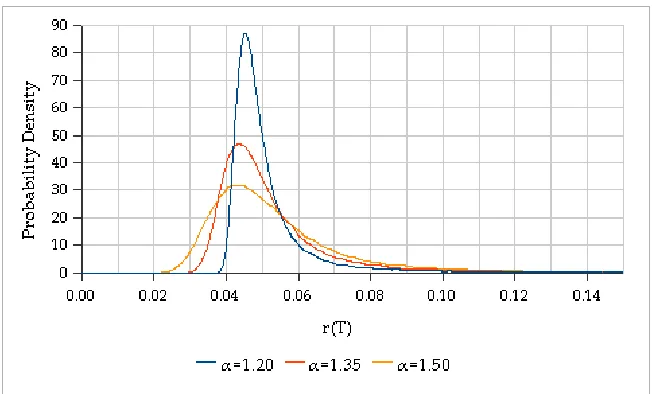
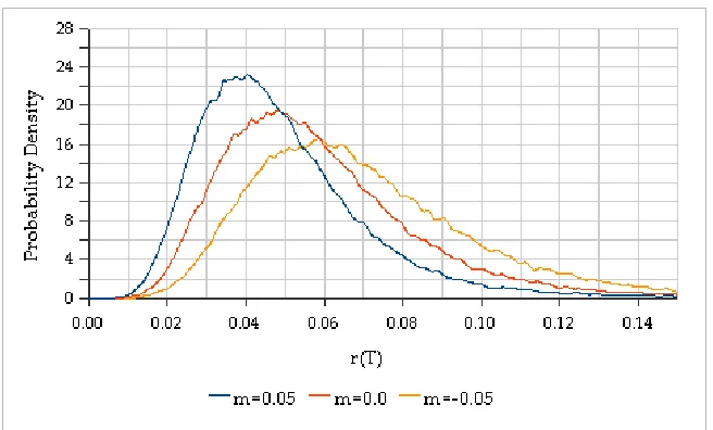
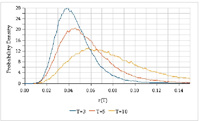
Results of the Monte Carlo simulation for constant drift𝜙 and a choice of other parameters are presented Figures 1-10 (𝑡 is set to zero). Figures 1-5 present the dependence of the probability distribution of 𝑟(𝑇) at 𝑇 = 5 on 𝛼, 𝜎, 𝑚 and 𝜙. Figure 6 shows the dependence on𝑇 itself. As can be seen from Figure 7, 𝑋 need not be too large. To understand the order of magnitude of 𝑋, note that the total intensity of Poisson processes starts off at 3𝑟(0)𝑋

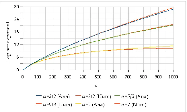
that is about 10 for 𝑟(0) = 0.03 and 𝑋 = 100, and corresponds to a time-step of about 0.1. To confirm the accuracy, the Laplace exponent is computed and displayed in Figure 8 for

𝛼= 3/2,5/3 and 2 for which closed form expressions are available from section 2.

An usual approach to understanding the distribution of a positive random variable is to compare it to a lognormal one. This can be done by computing the implied Black-Scholes volatility for a call or a put option on𝑟(𝑇) at various strikes, ignoring discounting and setting the underlying to E0(𝑟(𝑇)). The resulting volatility smile is plotted in Figure 9 for different

values of 𝛼. Figure 10 shows its dependence on 𝑇. The smile features are encouraging and further study is needed to confirm their applicability.

A

Semi-Analytics

Because affine processes have been well-studied, analytics of an 𝛼₋root process can be written down as a special case. However, for our purpose, it is simpler and more illuminating to derive the same starting with the pure-jump process

𝑑𝑟(𝑡) = [𝜙(𝑡)₋𝑚𝑋𝑟(𝑡)]𝑑𝑡+

∫ ∞

𝑧=0

ℎ𝑋(𝑧/𝑟(𝑡))𝑑𝑁(𝑑𝑧, 𝑡). (22)

Here ℎ𝑋(𝑥) = 0 for 𝑥 > 𝑋 given a large 𝑋 and ℎ𝑋(𝑥) = ℎ(𝑥) for 𝑥 ≤ 𝑋. This effectively

cuts off the integral over𝑧 at the higher end ensuring that the total intensity of the Poisson processes is finite. The object of interest is the following expectation value

𝐹𝑇(𝑟(𝑡), 𝑡)≡E𝑡

{

exp

[

−

∫ 𝑇

𝑡

𝑑𝑠𝑢𝑇(𝑠)𝑟(𝑠)

]}

. (23)

Its differential can be written down using Ito’s calculus leading to

∂𝐹𝑇

∂𝑡 + (𝜙−𝑚𝑋𝑟) ∂𝐹𝑇

∂𝑟 −𝑢𝑇𝑟𝐹𝑇 +𝑟

∫ ∞

0

𝑑𝑥[𝐹𝑇(𝑟+ℎ𝑋(𝑥), 𝑡)−𝐹𝑇(𝑟, 𝑡)] = 0. (24)

Integration variable 𝑧 is scaled to 𝑥=𝑧/𝑟(𝑡). The above can be solved with the ansatz

𝐹𝑇(𝑟(𝑡), 𝑡) = exp [−𝐴𝑇(𝑡)−𝐵𝑇(𝑡)𝑟(𝑡)]. (25)

Equating coefficients of 𝐹𝑇 independent of𝑟 and those linear in 𝑟 separately gives

𝑑𝐴𝑇(𝑡)

𝑑𝑡 +𝜙(𝑡)𝐵𝑇(𝑡) = 0, 𝑑𝐵𝑇(𝑡)

𝑑𝑡 −𝑚𝑋𝐵𝑇(𝑡) +𝑢𝑇(𝑡) +

∫ 𝑋

0

Consider now 𝑢𝑇(𝑡) = 𝑢(𝜏) as a function of 𝜏 = 𝑇 −𝑡 only. Then 𝐵𝑇(𝑡) = 𝐵(𝜏) is also a

function of 𝜏 only, satisfying 𝐵(0) = 0 and the differential equation

𝑑𝐵(𝜏)

𝑑𝜏 +𝑚𝑋𝐵(𝜏) =𝑢(𝜏) +

∫ 𝑋

0

𝑑𝑥_{1₋exp [₋ℎ(𝑥)𝐵(𝜏)]_}. (27)

With ℎ(𝑥) assumed to go to zero as 𝑥_{→ ∞}, the integrand above goes to zero as ℎ(𝑥)𝐵(𝜏), so that the above equation tends to be independent of 𝑋 for large 𝑋 if 𝑑𝑚𝑋/𝑑𝑋 =ℎ(𝑋).

A choice for 𝑚𝑋 with such a large 𝑋 behavior is 𝑚𝑋 =𝑚+

∫𝑋

0 𝑑𝑥ℎ(𝑥) (assuming ℎ(𝑥) is

integrable from 𝑥= 0). Equation for 𝐵(𝜏) then reads as in (3) in the limit 𝑋 _{→ ∞}. Given a solution for𝐵(𝜏) satisfying 𝐵(0) = 0, and 𝐴𝑇(𝑡) expressed as an integral of𝐵(𝜏), solution

for 𝐹𝑇(𝑟(𝑡), 𝑡) is as given in equation (2).

If 𝑢(𝜏) = 𝑢𝛿(𝜏₋0+) where 𝛿(𝜏 −0+) is a Dirac-delta function sitting just above 𝜏 = 0,

one obtains the Laplace transform E𝑡{exp [−𝑢𝑟(𝑇)]} of the probability density function of

𝑟(𝑇), or its negative logarithm known as the Laplace exponent. For this, equation (3) is solved for 𝐵(𝜏) in the absence of 𝑢(𝜏), but under the initial condition𝐵(0) =𝑢.

For ℎ(𝑥) =𝑎𝑥−1/𝛼

, 1< 𝛼 < 2, equation for 𝐵(𝜏) reads as in (4). The 𝑥₋integral in (3) is₋𝛼Γ(₋𝛼)𝑎𝛼_[𝐵(𝜏)]𝛼_{. Note that} ∫𝑋

0 𝑑𝑥ℎ(𝑥) =𝑎𝛼𝑋(𝛼 −1)/𝛼

/(𝛼₋1) diverges as𝑋 _{→ ∞}, but gets absorbed into𝑚𝑋. The𝛼 = 1 case is special. The𝑥−integral in (27) is−𝑎𝐵(𝜏) ln𝐵(𝜏)

up to terms linear in 𝐵(𝜏) that are taken care of by 𝑚𝑋 =𝑚+𝑎ln(𝑋/𝑎) +𝑎(1−𝛾) where

𝛾 is the Euler’s constant.

One may wonder whether an 𝛼₋root process can be defined for 𝛼 <1 as well. After all, the 𝑥₋integral in (27) is then finite as 𝑋 _{→ ∞} and is ₋𝛼Γ(₋𝛼)𝑎𝛼_[𝐵(𝜏)]𝛼

. However, the integral dominates the 𝑚𝑋𝐵(𝜏) term as 𝐵(𝜏) → 0, and solving for the Laplace exponent

with 𝑢(𝜏) = 0 and 𝐵(0) =𝑢 yields a 𝐵(𝜏) that does not go to zero as 𝑢_→0.

References

[1] S. Asmussen and J. Rosi´nski (2001), “Approximations of small jumps of L´evy processes with a view towards simulation”, Journal of Applied Probability 38, 482-493.

[2] J. Bertoin (2000), “Subordinators, L´evy Processes with no negative jumps and branch-ing processes”, MaPhySto Lecture Notes, Series 8.

[3] D. Brigo and A. Alfonsi (2005), “Credit default swap calibration and derivatives pricing with the SSRD stochastic intensity model ”, Finance and Stochastics 9, 29-42.

[4] P. Carr and L. Wu (2004), “Time-changed L´evy processes and option pricing”, Journal of Financial Economics 71, 113-141.

[5] D. Duffie, D. Filipovic and W. Schachermayer (2003), “Affine processes and applications in finance”, The Annals of Applied Probability 13, 984-1053.

Figure 1: Plots of the probability density functions for 𝛼 = 1.65,1.80 and 1.95. Other parameters chosen are 𝑇 = 5, 𝜎 = 0.04, 𝑚 = 0.01, 𝜙 = 0.006 and 𝑟(0) = 0.03. Number of Monte Carlo scenarios is one million and cutoff 𝑋 is 100.

Figure 3: Plots of the probability density functions for 𝜎 = 0.03,0.04 and 0.05. Other parameters chosen are 𝑇 = 5, 𝛼 = 1.80, 𝑚 = 0.01, 𝜙 = 0.006 and 𝑟(0) = 0.03. Number of Monte Carlo scenarios is 100,000 and cutoff 𝑋 is 100.

Figure 5: Plots of the probability density functions for 𝜙 = 0.003,0.006 and 0.009. Other parameters chosen are 𝑇 = 5, 𝛼 = 1.80, 𝜎 = 0.04, 𝑚 = 0.01 and 𝑟(0) = 0.03. Number of Monte Carlo scenarios is 100,000 and cutoff 𝑋 is 100.

Figure 7: Plots of the probability density functions for cutoff 𝑋 = 20,100 and 500. Other parameters chosen are 𝑇 = 5, 𝛼 = 1.80, 𝜎 = 0.04, 𝑚 = 0.01, 𝜙 = 0.006 and 𝑟(0) = 0.03. Number of Monte Carlo scenarios is 100,000.

Figure 8: Plots of the Laplace exponents computed analytically and numerically for 𝛼 = 3/2,5/3 and 2. Other parameters chosen are 𝑇 = 5, 𝜎 = 0.04, 𝑚 = 0.01, 𝜙 = 0.006 and

Figure 9: Plots of the volatility smiles for 𝛼= 1.65,1.80 and 1.95. Other parameters chosen are 𝑇 = 5, 𝜎= 0.04, 𝑚 = 0.01, 𝜙 = 0.006 and 𝑟(0) = 0.03. Number of Monte Carlo scenarios is 100,000 and cutoff𝑋 = 100.

Figure 10: Plots of the volatility smiles for 𝑇 = 3,5 and 10. Other parameters chosen are