SOFTWARE CONFIGURATION MANAGEMENT PRACTICE IN MALAYSIA

ARIMA METHOD WITH THE SOFTWARE MINITAB AND

EVIEWS TO FORECAST INFLATION

IN SEMARANG INDONESIA

1_WARDONO,2_{ARIEF AGOESTANTO,}3_{SITI ROSIDAH}

1_{Doctor, Department of Mathematics, Semarang State University, Indonesia}

2_{Magister, Department of Mathematics, Semarang State University, Indonesia}

3_{Student, Department of Mathematics, Semarang State University, Indonesia} E-mail: 1_{[email protected] ,}2_{[email protected],}3_{[email protected]}

ABSTRACT

Inflation is one of the indicators to see the economic stability of a region. The value of inflation in Semarang district on January 2014 - April 2016 unstable. Inflation which unstable will impede the economic development in Semarang district, therefore need to be undertaken against the value of the modeling inflation in the future with a method of ARIMA. The purpose of this study is to find a model ARIMA which appropriate to forecasting inflation in Semarang district and to know the forecasting inflation in Semarang district on May 2016 - April 2017 using Minitab and Eviews software. Minitab and Eviews are two statistical packages programs that both can be used to analyze the time series data. The next, the authors wanted to know which of these programs is more accurate than the other in estimating the value of inflation. The methods used in this study is a literature method i.e. authors collect, select and analyze readings related to the issues examined and methods documentation i.e. the author collected data in inflation on January 2010 - April 2016 in Semarang district. Based on the research obtained, the model appropriate to forecasting inflation in Semarang district is a model ARMA(2,1) or ARIMA(2,0,1). The results of the forecasting inflation at Semarang district using Minitab and Eviews software on May 2016 – April 2017 is stable enough. The best model to foresee the next period is ARMA(2,1) or ARIMA(2,0,1) model with software Eviews namely with the following equation :

= 1,3551 − 0,5756 + − 0,9789 .

The highest inflation occurred on September, October, and November 2016 and lowest Inflation occurred on May and June 2016.

Keywords:ARIMA, Minitab, Eviews, Forecast, Inflation

1. INTRODUCTION

In the economy of a region, inflation became an important thing that made the benchmark for economic growth, a factor of consideration in selecting the type of investment the investor, as well as the deciding factor for the Government in formulating fiscal policy, monetary or non-monetary.

Inflation is symptoms indicating the increase in the level to the general price lasting continuously (Mishkin, 2001). According to BPS, as quoted by Berlian, Wilandari & Yasin (2014), inflation is one of the indicators to see the economic stability of a region or an area that shows the development of

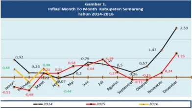
prices of goods and services in general are calculated from the consumer price index.

Source: http://semarangkab.bps.go.id

On the graph to see that the value of the monthly inflation in Semarang District in January 2014 until April 2016 is fluctuation. This shows that inflation in Semarang District is unstable. The stability of inflation is a prerequisite for sustainable economic growth, which in turn provide benefits to an increase in welfare of society. The importance of controlling inflation is based on the consideration that the high inflation and unstable give negative effects to the socio-economic condition of the community (http://www.bi.go.id).

Because inflation give impact on the economy in Semarang district, then it needs to be done against the inflation rate modeling in the future so as to determine the steps that need to be prepared in the face of economic conditions ahead are influenced by inflation with ARIMA method.

A general model of time series Autoregressive (AR), the Moving Average (MA) and Autoregressive Moving Average (ARMA) is often used to model the financial and economic data assuming stationarity against range (homokedastisitas). Therefore, it takes a time series model that can model the most economic and financial data by retaining data heteroskedastisitas (Engle, 2001).

Along with the advancement of information technology with use some help computers allow activities forecasting at the time of this can be conducted easily. The advance of software the thriving now create many software applications specifically applied for the forecasting (Santoso, 2009).

At the moment there are a variety of computer applications software that can help in the process of forecasting data easily, quickly and accurately, especially if using analysis of time series (Dwitanto, 2011). Technology computer software that can be used to analyse the forecasting using method time series is Minitab and Eviews software. Minitab and Eviews is software that can be used to analyze economic forecasting with complete and easy enough, for example, inflation forecasting, macroeconomic forecasting and sales forecasting.

EViews(Econometric Views) is a statistical package for Windows, used mainly for time-series oriented macro-econometric analysis. EViews can be used for general statistical analysis and econometric analyses, such as time series estimation and forecasting, cross-section and panel data analysis. EViews combines spreadsheet and

relational database technology found in statistical software, and uses a Windows GUI. EViews relies heavily on a proprietary and undocumented file format for data storage. However, for input and output it supports numerous formats, including databank format, Excel formats, PSPP/SPSS, DAP/SAS, Stata, RATS, and TSP. EViews can access ODBC databases. EViews file formats can

be partially opened by gretl.

(https://en.wikipedia.org/wiki/EViews)

According to Simarmata, as quoted by Hadijah (2013), Minitab is a computer program that is designed to perform processing of statistics. Minitab also provides regression analysis (simple regression analysis as well as multiple regression), multivariate analysis (factor analysis, discriminan analysis, cluster analysis, principal component), qualitative data analysis, time series analysis, and some nonparametric analysis (Iriawan, 2006).

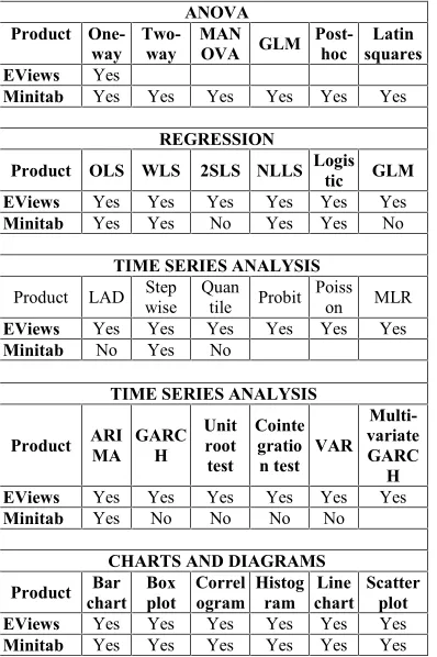
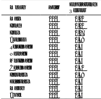
There are some differences of ability Eviews and Minitab in frame of statistical analysis (https://en.wikipedia.org) , ie :

Table 1. Differences Of Ability Eviews And Minitab In Frame Of Statistical Analysis

ANOVA Product

One-way Two-way MANOVA GLM Post-hoc squaresLatin EViews Yes

Minitab Yes Yes Yes Yes Yes Yes

REGRESSION

Product OLS WLS 2SLS NLLS Logis_tic GLM EViews Yes Yes Yes Yes Yes Yes Minitab Yes Yes No Yes Yes No

TIME SERIES ANALYSIS

Product LAD Step_wise Quan_tile Probit Poiss_on MLR EViews Yes Yes Yes Yes Yes Yes Minitab No Yes No

TIME SERIES ANALYSIS

Product ARI_MA GARC_H Unitroot test

Cointe gratio n test VAR

Multi-variate GARC

H EViews Yes Yes Yes Yes Yes Yes

Minitab Yes No No No No

CHARTS AND DIAGRAMS

Product Bar_chart Box_plot Correl_ogram Histog_{ram chart}Line Scatter_plot EViews Yes Yes Yes Yes Yes Yes Minitab Yes Yes Yes Yes Yes Yes

paper will discuss the accuracy of them (Eviews 8.1 and Minitab 16 packages) in forecasting using ARIMA. Minitab and Eviews are two statistical packages programs that both can be used to analyze the time series data. The next, the authors wanted to know which of these programs is more accurate than the other in estimating the value of inflation.

Rokhaniyah and Nugroho , in their study which aims to identify the occurrenceof fly paper on the city and county government spending in Indonesia, in 2012-2014. In this case, the dependent variable used is the shopping area while the independent variable is revenue (R), the General Allocation Fund (GAF) , the Special Allocation Fund (SAF) and a dummy, to distinguish the city /county Java and Outside Java. This research uses software Eviews 6. The objective of the study (Ikrima and Muharam,2014) was to analyze the Greece’s crisis impacts toward the movement of Islamic stock prices in Indonesia, Malaysia, USA, and Europe. Moreover, this study also analyzed co-integration and contagion effect which occurred during the period. VAR (Vector Auto Regressive) and VECM (Vector Error Correction Model) with eviews 6 were used to test the hypothesis as the statistical analysis tools. Syahnur’s Research (2013) aims to: determine the extent of inflation, economic growth, and investments against unemployment in the province of Central Java. Data analysis technique used is the panel data regression analysis and path analysis with the help of a computer program Eviwes 6.0.

This article (Waryanto and Millafati,2006) will discuss the improvement, which has been made in the tranformation of ordinal data to an interval data at least with data scale. In order to perform that task, a transformation program, this program is designed by using the makro Minitab. This program is able to transform ordinal data in Likert scale to an interval data, at least with scale 3 category. In addition, this program is also capable in transforming data wich is not completely filled out. Syafii and Noveri (2013) conducted a study of short-term or daily electricity load curve forecasting use ARIMA through the stages: checking the data patterns, identifying models of stationary test variance and mean, parameter estimation and measurement of the accuracy of the model using MAPE.

Based on it, the formulation of problems in this final project is a model of ARIMA where appropriate for forecasting inflation in Semarang using Minitab and Eviews software? and what is

the result of inflation forecasting in Semarang in may 2016 – April 2017 using Minitab and Eviews software?. The purpose of this study is to find out which exact model of ARIMA for forecasting inflation in Semarang and to know the results of the forecasting inflation at Semarang in may 2016 – April 2017 using Minitab and Eviews software.

2. RELEVANT STUDIES 2.1 Inflation

According to Sukirno (2008), inflation is defined as a process of rising prices in an economy. According to Sunariyah (2006), inflation is the increase in the prices of goods and services on an ongoing basis. According to Tandelilin (2010), inflation is the trend of increased prices of products as a whole.

Inflation according to the condition of the Puthong (2002), based on their nature is divided into four main categories of: Creeping Inflation, Galloping Inflation, High Inflation, and Hyper Inflation.

Inflation is the tendency of prices to rise in general and continuously. Low inflation rate will reduce price variability and increase efficiency in the economy (Ball and Mankiw, 1994a, 1994b, 1995) but based on the model of nominal wage rigidity is obtained that efficiency in the economy will be reduced if inflation is too low (Akerlof, Dickens and Perry, 1996) , Therefore the optimal inflation rate should be made so that it will lead to economic stability. Based on research Muhson, A. (1999), with the regression analysis method enter obtained model the relationship between the rate of inflation with the money supply, exchange rate, interest rate and national income are together there is a significant relationship between the amount of money in circulation , exchange rate, interest rate and national income and the inflation rate in Indonesia.

growth. Third, the domestic inflation rate higher than the rate of inflation in neighboring countries make real domestic interest rates become uncompetitive so as to put pressure on the rupiah.

Low and stable inflation in the long term will support sustainable economic growth (suistanable growth) because the inflation rate is positively correlated with the fluctuation. When inflation is high, fluctuation also increased, so that people feel uncertain with the inflation rate will occur in the future. As a result, long-term interest rates will rise because of the high risk premium due to inflation.

2.2 Forecasting

Forecasting is a estimated that will occur in the future, while the plan is the determination of what will be done in the time to come (Subagyo, 1986). In making forecasts to be able to have minimised the influence of uncertainty. In other words, forecasting the forecasts can get aim at minimising mistakes predict (Forecast error) which is typically measured by the Mean Square Error (MSE), the Mean Absolute Error (MAE) and so (Subagyo, 1986).

2.3 Time Series Analysis

Time series analysis is a quantitative method to determine the pattern of past data that has been collected on a regular basis, for forecasting the future. While time series data is a statistical data compiled on the basis of the time of the incident. Could be the year, quarter, month, week, and so on (Soejoeti, 1987). Time series data i.e. data collected from time to time to see the development of an activity, where when the data described will show fluctuations and can be used for the base withdrawal trends that can be used for basic forecasting is useful for basic planning and withdrawal of the conclusions (Supranto, 2001).

According to Makridakis, & Wheelwrigt McGee (1995) time series data pattern can be differentiated into four types, namely the pattern of horizontal (H), the seasonal Pattern (S), (C) cyclical Pattern, and the pattern of trend (T). According to Soejoeti (1987) based on the historical value of his observation time runtun is distinguished into two, namely determninastic time series and stochastic time series. According to Spiegel & Stephens (2007), based on movement or variation time series consists of three kinds of patterns, namely: the long-term movement or trend, movement/ cyclical variation and movement/seasonal variations.

Many empirical time series behave as though they have no fix mean. Even so, they exhibit

homogeneity in the sense that, apart from local level, or perhaps local level and trend, one part of the series behaves much like any other part. Model which describe such homogeneous nonstationary behavior can be obtained by supposing some suitable differenceof the process to be stationary. The properties of the important class of models for which the th difference is a stationary mixed autoregressive-moving average (ARIMA) process.

2.4. Autoregressive (AR) processes

A time series{ }is said to be an autoregressive process of order (abbreviated AR( )) if it is a weighted linear sum of the past values plus a random shock so that :

= + + ⋯ + + (1)

where { }denotes a purely random process with zero mean and variance . Using the backward shift operator , such that = , the AR( ) model may be written more succinctly in the form

( ) = (2)

where ( ) = 1 − − − ⋯ − is a

polynomial in of order . The properties of AR processes defined by (1) can be examined by looking at the properties of the function . As is an operator, the algebraic properties of have to be investigated by examining the properties of ( ), say, where denotes a complex variable, rather than by looking at ( ). It can be shown that (2) has a unique causal stationary solution provided that the roots of ( ) = 0 lie outside the unit circle. This solution may be expressed in the form

= (3)

for some constants such that∑ < ∞. The above statement about the unique stationary solution of (2) may be unfamiliar to the reader who is used to the more customary timeseries literature. The latter typically says something like “an AR process is stationary provided that the roots of

( ) = 0lie outside the unit circle”. This will be

good enough for most practical purposes but is not strictly accurate; for further remarks on this point, see Brockwell and Davis (1991).

The simplest example of an AR process is the first-order case given by

The time-series literature typically says that an AR(1) process is stationary provided that| | < 1. It is more accurate to say that there is a unique stationary solution of (4) which is causal, provided

that | | < 1. The ac.f. of a stationary AR(1)

process is given by

= + +⋯+ (5)

for = 0,1,2, . ..., where = 0 . Notice that the

AR model is typically written in mean-corrected

form with no constant on the right-hand side of (1). This makes the mathematics much easier to handle. A useful property of an AR( ) process is that it can be shown that the partial ac.f. is zero at all lags greater than . This means that the sample partial ac.f. can be used to help determine the order of an AR process (assuming the order is unknown as is usually the case) by looking for the lag value at which the sample partial ac.f. ‘cuts off’ (meaning that it should be approximately zero, or at least not significantly different from zero, for higher lags).

2.5. Moving average (MA) processes

A time series{ }is said to be a moving average process of order (abbreviated MA( )) if it is a weighted linear sum of the last random shocks so that

= + +⋯+ (6)

where { } denotes a purely random process with zero mean and constant variance . (6) may alternatively be written in the form

= ( ) (7)

where ( ) = 1 − − −⋯− is a

polynomial in of order . Note that some authors (including Box et al., 1994) parameterize an MA process by replacing the plus signs in (6) with minus signs, presumably so that ( )has a similar form to ( )for AR processes, but this seems less natural in regard to MA processes. There is no difference in principle between the two notations but the signs of the values are reversed and this can cause confusion when comparing formulae from different sources or examining computer output.

It can be shown that a finite-order MA process is stationary for all parameter values. However, it is customary to impose a condition on the parameter values of an MA model, called the invertibility condition, in order to ensure that there is a unique MA model for a given ac.f. This condition can be explained as follows. Suppose that { }and { }

are independent purely random processes and that

∈ (−1,1). Then it is straightforward to show that

the two MA(1) processes defined by

= + and = + have

exactly the same autocorrelation function (ac.f.). Thus the polynomial ( ) is not uniquely determined by the ac.f. As a consequence, given a sample ac.f., it is not possible to estimate a unique MA process from a given set of data without putting some constraint on what is allowed. To resolve this ambiguity, it is usually required that the polynomial ( ) has all its roots outside the unit circle. It then follows that we can rewrite (6) in the form

− = (8)

for some constants such that| | < ∞. In other words, we can invert the function taking the sequence to the sequence and recover from present and past values of by a convergent sum. The negative sign of the -coefficients in (8) is adopted by convention so that we are effectively rewriting an MA process of finite order as an AR(∞) process. The astute reader will notice that the invertibility condition (roots of ( )lie outside unit circle) is the mirror image of the condition for stationarity of an AR process (roots of ( ) lie outside the unit circle).

The ac.f. of an MA( ) process can readily be shown to be

=

⎩ ⎪ ⎨ ⎪

⎧ 1, = 0

∑ , = 1,2, … ,

0, >

(9)

where = 1. Thus the ac.f. ‘cuts off’ at lag . This property may be used to try to assess theorderof the process (i.e. What is the value of ?) by looking for the lag beyond which the sample ac.f. is not significantly different from zero.

regression on the remote past is useless for prediction purposes, then the process is said to benondeterministic(or purely indeterministic or regular or stochastic).

The connection with MA processes is as follows. It can be shown that the non-deterministic part of the Wold decomposition can be expressed as an MA process of possibly infinite order with the requirement that successive values of the sequence are uncorrelated rather than independent as assumed by some authors when defining MA processes. Formally, any stationary non-deterministic time series can be expressed in the form

= (10)

where = 1and ∑ < ∞, and { }denotes a purely random process (or uncorrelated white noise) with zero mean and constant variance, , which is uncorrelated with the deterministic part of the process (if any). The{ }are sometimes called

innovations, as they are the one-step-ahead forecast errors when the best linear predictor is used to make one-step ahead forecasts. The formula in (10) is an MA(∞) process, which is often called the Wold representationof the process. However, note that the latter terms are used by some writers when the ’s are independent, rather than uncorrelated, or when the summation in (10) is from−∞to+∞, rather than 0 to ∞. Of course, if the ’s are normally distributed, then zero correlation implies independence anyway and we have what is sometimes called a Gaussian linear process.

MA(∞) representation of a stochastic process involves an infinite number of parameters which are impossible to estimate from a finite set of data. Thus it is customary to search for a model that is a parsimonious approximation to the data, by which is meant using as few parameters as possible. One common way to proceed is to consider the class of mixed ARMA processes as described below.

2.6. ARMA processes

A mixed autoregressive moving average model with autoregressive terms and moving average terms is abbreviated ( , )and may be written as :

( ) = ( ) (11)

where ( ), ( ) are polynomials in of finite order , ,respectively. This combines (2) and (7). Equation (11) has a unique causal stationary solution provided that the roots of ( ) = 0 lie

outside the unit circle. The process is invertible provided that the roots of ( ) = 0 lie outside the unit circle. In the stationary case, the ac.f. will generally be a mixture of damped exponentials or sinusoids.

The importance of ARMA processes is that many real data sets may be approximated in a more parsimonious way (meaning fewer parameters are needed) by a mixed ARMA model rather than by a pure AR or pure MA process. We know from the Wold representation that any stationary process can be represented as a MA(∞) model, but this may involve an infinite number of parameters and so does not help much in modelling. The ARMA model can be seen as a model in its own right or as an approximation to the Wold representation in (10). In the latter case, the generating polynomial in B ,which gives (10) , namely

( ) =

may be of infinite order, and so we try to approximate it by a rational polynomial of the form

( ) = ( )_{( )}

which effectively gives the ARMA model.

This subsection takes a more thorough look at some theoretical aspects of ARMA processes (and hence of pure AR and MA processes by putting or equal to one). Time-series analysts typically say that this equation is an ARMA( , )

process. However, strictly speaking, the above equation is just that - an equation and not a process. In contrast, the definition of a process should uniquely define the sequence of random variables { }. Like other difference equations, (11) will have infinitely many solutions (except for pure MA processes) and so, although it is possible to say that any solution of (11) is an

ARMA( , ) process, this does not of itself

uniquely define the process.

Consider, for example, the AR(1) process, for which :

= + (12)

for = 0, ±1, ±2, …. As noted earlier, it is

solutions. For example, the reader may check that the following process is a solution to (12) :

= +

where denotes a constant.If we take to be zero, then we obtain the unique stationary solution, but for any other value of , the process will not be stationary. However, it is readily apparent that the general solution will tend to the stationary solution as → ∞.In this regard the question of whether or not the equation is

stable becomes important. The property of stability is linked to stationarity. If we regard (12) as a linear filter for changing an input process

{ } to an output process { }, then it can be shown that the system is stable provided that

| | < 1. This means that the effect of any

perturbation to the input will eventually die away.This can be used to demonstrate that any deviation from the stationary solution will also die away.Thus the general solution tends to the stationary solution as increases.

A stationary ARMA process may be written as an MA(∞) process by rewriting (11) in the form

= ( )_{( )}

and expanding / as a power series in . For a causal process, the resulting representation may be written in the same form as the Wold representation in (10), or (3), namely

= (14)

or as

= ( ) (15)

where ( ) = + + +⋯. A finite

MA process is always stationary as there is a finite sum of ’s. However, for an infinite sequence, such as that in (14), the weighted sum of Z ’s does not necessarily converge. From (14), it can readily be shown that

Variance( ) = (16)

and so we clearly require ∑ <∞ for the variance to be finite.

It may not be immediately obvious why it may be helpful to re-express the ARMA process in (11) as an MA(∞) process in the form (14). In fact, the

MA(∞) representation is generally the easiest way to find the variance of forecast errors. For computing point forecasts, it may also be helpful to try to re-express the process as an AR(∞) process.It turns out that, if the process is invertible, then it is possible to rewrite (11) in the form of (8) as

( ) = (17)

where, by convention, we take ( ) = 1 − ∑ , and where∑ < ∞so that the ’s are summable.

The ARMA process in (11) has ( ) and ( )

of finite order, whereas when a mixed model is expressed in pure MA or AR form, the polynomials

( ) and ( ) will be of infinite order.We have seen that an ARMA process is stationary if the roots of ( ) = 0 lie outside the unit circle and invertible if the roots of ( ) lie outside the unit circle.We can find corresponding conditions in terms of ( )or ( ).

2.7. ARIMA processes

We now reach the more general class of models which is the title of the whole of this section. In practice many (most?) time series are nonstationary and so we cannot apply stationary AR, MA or ARMA processes directly. One possible way of handling non-stationary series is to apply differencing so as to make them stationary. The first differences, namely( − ) = (1 − )

may themselves be differenced to give second differences, and so on. Thedth differences may be written as(1 − ) . If the original data series is differenceddtimes before fitting an ARMA( , ) process, then the model for the original undifferenced series is said to be an ARIMA( , , ) process where the letter ‘I’ in the acronym stands for integrated and denotes the number of differences taken.

Mathematically, (11) is generalized to give:

( )(1 − ) = ( ) (18)

The combined AR operator is now (1 − ) . If we replace the operator in this expression with a variable , it can be seen straight away that the function ( )(1 − ) has roots on the unit circle (as(1 − ) = 0when = 1) indicating that the process is non-stationary – which is why differencing is needed.

equals one, then the model reduces to an ARIMA(0,1,0) model, given by

− = (19)

This is obviously the same as the random walk model which can therefore be regarded as an ARIMA(0,1,0) model.

When fitting AR and MA models, the main difficulty is assessing the order of the process rather than estimating the coefficients (the ’s and ’s). With ARIMA models, there is an additional problem in choosing the required order of differencing. Some formal procedures are available, including testing for the presence of a unit root, but many analysts simply difference the series until the correlogram comes down to zero ‘fairly quickly’. First-order differencing is usually adequate for non-seasonal series, though second-order differencing is occasionally needed. Once the series has been made stationary, an ARMA model can be fitted to the differenced data in the usual way.

2.8. Determining The Best Model

To determine the best model of several models of ARIMA can be used several criteria, among others: criteria for Mean Square Error (MSE), Akaike's Information Criterion (AIC) and Schwartz's Bayesian Criterion (SBC). The best model was chosen that the value of the smallest message (Aswi & Sukarna, 2006). Some of the ways used to measure i.e. forecasting errors as follows: Mean Square Error (MSE), the Root Mean Square Error (RMSE), the Mean Absolute Error (MAE), and Mean Absolute Percentage Error (MAPE). In addition, the accuracy of a forecast also needs to be based on: the bias proportion variance proportion covariance, and proportion. The value of forecasting will say "good/accurate approach" If the bias proportion variance proportion, and fairly small but relatively high proportion covariance (Pindyck Rubinfeld &, 1991).

3. METHOD

The scope of the research in this study is the data of inflation in January of 2010 to April 2016 in Semarang district. The inflation data will be made the value of forecasting in May 2016 until April 2017. In this study, data retrieved from website BPS Semarang district that address of the site that is as follows: http://semarangkab.bps.go.id.

The methods used in this study consists of several stages, namely, methods of literature and methods of documentation. The methods of the literature is one method of finding the information

obtained from the book module, reference books, scientific journals, and scientific essay. This is done to provide the Foundation of teroritis and solving problems posed in this study. Method documentation is a method of data collection conducted in institutions or establishments that present the data in question. In this study, data obtained from the website of the Central Bureau of Statistics (BPS), that the general inflation in Semarang in January 2010 until April 2016. The inflation data is data ready to use so that authors do not do a calculation of inflation. This data is then processed using the most suitable forecasting method based on the pattern of the data because the data time series. The data will be analyzed using the method of ARIMA using Minitab 16 and Eviews 8.1 software.

There are several stages in the runtun analysis time: the first step that is the identification of the model. At this stage we choose the right model that can represent the series of observations. Model identification is performed by making a plot runtun time and uses the parameters a little might be called the principle of parsimony. Steps to identify model runtun time is as follows: create a plot, makes the time ACF runtun (autocorrelation function) and the PACF (partial autocorrelation function) and check out the stationary data (Hendikawati, 2015).

The second step namely estimation model. At this stage, after having obtained the results of the model parameter estimation, conducted a test of the significance of the parameters. This test is used to determine whether a parameter AR (p), differencing (d), MA (q), and constants are significant or not. If these parameters are significant, then the model is worth used. If the coefficients estimated from model dipih does not meet the conditions of a particular mathematical inequality, then the model is rejected (Hendikawati, 2015).

The third step, namely diagnostic checking. On diagnostic testing done checking to see if the selected model is already pretty well statistically. By looking at the results of fak and fakp plots of residual model, can be known of the existence of autokolerasi and partial correlation on the residual. A good forecasting model is that there is no autokolerasi and partial correlation on the residual. Models that do not go beyond this diagnostic test will be rejected (Hendikawati, 2015).

selected. Forecasting is an activity to predict what will happen in the future.

4. RESULTS AND DISCUSSION

The data analyzed are data on inflation in January of 2010 to April 2016 in Semarang district. Data analysis using Minitab and Eviews software.

Research results with Software Minitab i.e. the first phase is the identification of the model. At this stage identification model that is the first step is to make a plot of the data graphically.

72 64 56 48 40 32 24 16 8 1 4 3 2 1 0 -1 Index In fla si

Time Series Plot of Inflasi

Figure 2. Time Series Plot For Inflation Based on Figure 2 is seen that data pattern already formed stationary, the second Step is making the ACF and PACF.

18 16 14 12 10 8 6 4 2 1.0 0.8 0.6 0.4 0.2 0.0 -0.2 -0.4 -0.6 -0.8 -1.0 Lag Au to co rr el at io n

Autocorrelation Function for Inflasi

(with 5% significance limits for the autocorrelations)

Figure 3. The Graph Of The AutocorrelationFunction

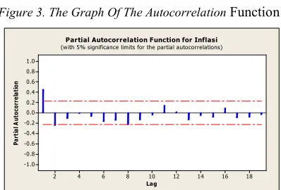
18 16 14 12 10 8 6 4 2 1.0 0.8 0.6 0.4 0.2 0.0 -0.2 -0.4 -0.6 -0.8 -1.0 Lag Pa rt ia lA ut oc or re la tio n

Partial Autocorrelation Function for Inflasi

(with 5% significance limits for the partial autocorrelations)

Figure 4. The Graph Of The Partial Autocorrelation Function

Based on Figure 3 looks that the graph is disconnected at lag 1. This is because the value of the lag 1 out from the boundary line and the value of lag 2 is close to zero, so the estimated model showed the process of MA(1). Figure 4 shows that the knowable order autoregerssive which might formed (significant). Seen that lag lag 1 and 2 only, whereas the partial lag autokolerasi next tend to approach zero or insignificant. Then the estimated model is formed is the process of AR(2).

Based on the results from the model identification charts ACF and PACF can be inferred that the model while that form is AR(2) or ARIMA(2,0,0), MA(1) or ARIMA(0,0,1) and ARMA(2,1) or ARIMA (2,0,1). Final The second stage i.e. the estimation model. Estimates of Parameters

Table 2. Models Of ARMA(2,0,0) Or AR(2)

From Table 2 is obtained probability value AR(1) in the table the Final Estimates of Parameters, namely in the amount of 0.000. Because the probability value = 0.000 < α = 0.05 then parameter AR(1) significant. The obtained probability value is also an AR(2) in the table the Final Estimates of Parameters i.e. of 0.024. Because the value of the probability = 0.024 < α = 0.05 then parameter AR(2) significant. The obtained probability value Constant also in the table of Final Estimates of Parameters, namely in the amount of 0.000. Because the probability value = 0.000 α = 0.05 < then Constant parameter is significant. Because the parameter of AR(1), AR(2) Constant are significant then models ARIMA (2,0,0) or AR(2) can be inserted into a likely model.

Table 3. Models Of ARIMA(0,0,1) Or MA(1)

From Table 3 probability values obtained MA(1) in the table the Final Estimates of Parameters, namely in the amount of 0.000. Because the probability value = 0.000 < α = 0.05 then MA(1) parameters significant. The obtained probability

Type Coef SE Coef T P

AR 1 0,5894 0,1148 5,13 0,000

AR 2 -0,2637 0,1148 -2,30 0,024

Constant 0,31450 0,0677 4,65 0,000

Mean 0,4664 0,1003

Type Coef SE Coef T P

MA 1 -0,5058 0,1040 -4,86 0,000

Constant 0,4641 0,1030 4,50 0,000

value Constant also in the table of Final Estimates of Parameters, namely in the amount of 0.000. Because the probability value = 0.000 < α = 0.05

then Constant parameter is significant. Because the parameters of the MA(1) Constant and significant then models ARIMA (0,0,1) or MA(1) it can be inserted into the possibility of a model. Final Estimates of Parameters ie :

Table 4. Models Of ARIMA(2,0,1) Or ARMA(2,1)

From Table 4 is obtained probability value AR(1) in the table the Final Estimates of Parameters, namely in the amount of 0.000. Because the probability value = 0.000 < α = 0.05 then parameter AR(1) significant. The obtained probability value is also an AR(2) in the table the Final Estimates of Parameters, namely in the amount of 0.000. Because the probability value = 0.000 < α = 0.05 then parameter AR(2) significant. Probability value also obtained an MA(1) in the table the Final Estimates of Parameters, namely in the amount of 0.000. Because the probability value = 0.000 < α = 0.05 then MA(1) parameters significant. The obtained probability value Constant also in the table of Final Estimates of Parameters, namely in the amount of 0.000. Because the probability value = 0.000 < α = 0.05 then Constant parameter is significant. Because the parameter of AR(1), AR(2), MA(1) Constant and significant then models ARIMA(2,0,1) or ARMA(2,1) it can be inserted into the possibility of a model.

The next step is done best by doing a model election overfitting. Following are the results of overfitting some possible models of ARIMA.

Table 5. Overfitting Models Arima Using Software Minitab

Model Significant SS MS

AR 2 Yes 25,3650 0,3475

MA 1 Yes 26,3912 0,3556

ARMA (2,1) Yes 22,1428 0,3075

Based on Table 5 shows that the best model is obtained that is ARMA(2,1), due to the significant parameter values and the value of the model SS and MS are smaller than model AR(2) and MA(1).

The third stage i.e. diagnostic checking. Minitab output showing test results Ljung-Box, Ljung-Box test used to detect the existence of a correlation between residual (Iriawan, 20016).

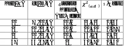
Table 6. Summary Of Test Result Ljung-Box-Pierce Models ARMA(2,0,1) Or ARMA(2,1)

Summary of the results in Table 6 shows that in the lag 12 value statistics Ljung-Box-Pierce = 10.3 < _{( %, )}= 15,507 means that until the lag 12, the conclusions that can be drawn is no correlation between residual at lag q with residual at lag 12. Similarly, for lag 24, 36 and 48 value statistics Ljung-Box-Pierce < _{( %, )}, _{( %, )}, and

( %, ). This means that the residual on residual

t with lag on (until) 48, no lag between mutually correlated lag. This means that the residual ARMA(2,1) are qualified white noise.

Based on the results of a test of the independence of the ARMA(2,1) model, residual residual model has independent, then the model ARMA(2,1) has been used to perform divination.

The fourth stage that is forecasting. After a diagnostic checking the next step is to do forecasting by using models that have been chosen, namely ARMA(2,1) or ARIMA(2,0,1).

Forecasts from period 76 95% Limits

Table 7. Inflation Data Forecast Results In Semarang District

Period Forecast Lower _ActualUpper

77 -0.14958 -1.23674 0.93758

78 0.15257 -1.00898 1.31412

79 0.39486 -0.76890 1.55861

80 0.54926 -0.66103 1.75955

81 0.61903 -0.65858 1.89664

82 0.62470 -0.70355 1.95295

83 0.59223 -0.76060 1.94506

84 0.54495 -0.81498 1.90488

85 0.49958 -0.86094 1.86010

86 0.46531 -0.89545 1.82607

87 0.44499 -0.91698 1.80696

88 0.43717 -0.92627 1.80061

Lag ( ) df (K-k) Statistik

Ljung-Box-Pierce

( , ) P-Value

12 8 (12-4) 10,3 15,507 0,247

24 20 (24-4) 21,2 31,410 0,388

36 32 (36-4) 32,7 46,194 0,434

48 44 (48-4) 37 60,481 0,762

Type Coef SE Coef T P

AR 1 1.3551 0.0989 13.70 0.000

AR 2 -0.5756 0.0984 -5.85 0.000

MA 1 0.9789 0.0503 19.47 0.000

Constant 0.101996 0.004030 25.31 0.000

Based on the Table 7 shows that inflation data forecast results in Semarang in may 2016, i.e.-0.14, June 2016, i.e. 0.15, July 2016, i.e. 0.39, August 2016, i.e. 0.55, September 2016, 0.62, i.e. October 2016, 0.62, i.e. November 2016, i.e. 0.60, in December 2016, i.e. 0.54 in January, 2017, that is 0.50, February 2017 i.e. 0.47, March 2017, i.e. 0.44 and April 2017, i.e. 0.44.

Research results with Software Eviews i.e. the first phase is the identification of the model. At this stage identification model that is the first step is to create the chart.

Figure 5. Inflation Chart

Based on Figure 5 above seen that indication data stationary. It is visible from its graph is around the average or in other words the average and variance is constant. The second step of the test, namely stasionerity.

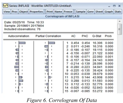
Figure 6. Correlogram Of Data

Based on the appearance of the Figure 6 shows that the autocorrelation graph shows disconnected immediately headed to zero after a lag of 1. This is

also indicated by the third column, whose value starts from 0.454 and next value tends to be close to zero. This shows indication data stationary. The third step, namely unit root test.

Figure 7. Unit Root Test Results

Based on the Figur 7 shows that value at α = 5% is -2.9012 smaller than the value of the statistic t of the ADF Test statistics "i.e. -5.6055 (notice the value used is the absolute value) this indicates that the data is already stationary so no need for data differencing.

The second stage i.e. the estimation model. At this stage it will do a test of the significance of the parameters.

Figure 8. The Results Of The Estimation Model Of ARIMA(2,0,0) Or AR(2)

parameter is significant. Because the parameter of AR AR (1), (2) Constant and significant then models ARIMA(2,0,0) or AR(2) can be inserted into a likely model.

Figure 9. The Results Of The Estimation Model Of ARIMA(0,0,1) Or MA(1)

From the obtained probability value Figure 9 MA(1) in the table the Final Estimates of Parameters, namely in the amount of 0.000. Because the probability value = 0.000 < α = 0.05 then MA(1) parameters significant. The obtained probability value Constant also in the table of Final Estimates of Parameters, namely in the amount of 0.000. Because the probability value = 0.000 < α = 0.05 then Constant parameter is significant. Because the parameters of the MA(1) Constant and significant then models ARIMA(0,0,1) or MA(1) it can be inserted into the possibility of a model.

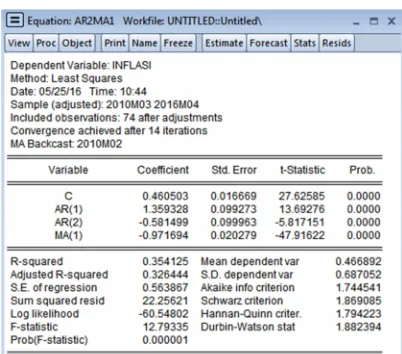
Figure 10. The Results Of The Estimation Model Of ARIMA(2,0,1) Or ARMA(2,1)

From Figure 10 obtained value of the probability of the AR(1) in the table the Final Estimates of Parameters, namely in the amount of 0.000. Because the probability value = 0.000 < α = 0.05

then parameter AR(1) significant. The obtained probability value is also an AR(2) in the table the Final Estimates of Parameters, namely in the amount of 0.000. Because the probability value = 0.000 < α = 0.05 then parameter AR(2) significant. Probability value also obtained an MA(1) in the table the Final Estimates of Parameters, namely in the amount of 0.000. Because the probability value = 0.000 < α = 0.05 then MA(1) parameter significant.

Table 8. Overfitting Models Arima Using Software Eviews

The obtained probability value Constant also in the Table 6 of Final Estimates of Parameters, namely in the amount of 0.000. Because the probability value = 0.000 < α = 0.05 then Constant parameter is significant. Because the parameter of AR(1), AR(2), MA(1) Constant and significant then models ARIMA(2,0,1) or ARMA(2,1) it can be inserted into the possibility of a model.

The next step is done best by doing a model election overfitting. Following are the results of overfitting some possible models of ARIMA.

Based on Table 8 shows that the best model is obtained that is ARMA(2,1), due to the significant parameter values and the value of SSE, AIC and the SBC the smaller model from model AR(2) and MA(1).

The third stage i.e. diagnostic checking. At this stage of the testing done to see if the selected model is already pretty well statistically. The trick is to test whether the residual estimation results already are white noise. When residualnya already white noise means the model is just right (Winarno, 2011).

Model Significant SSE AIC SBC

AR(2) Yes 0,597214 1,846614 1,940022

MA(1) Yes 0,597191 1,832804 1,894134

Figure 11. Correlogram Of Residual ARIMA(2,0,1) Or ARMA(2,1)

On the basis of the Table 11 it appears that residual already are random. This is shown by the bar graph which are all located in Bartlett's line. From the independence of the residual test results, a model of ARMA(2,1) are qualified white noise.

Based on the results of a test of the independence of the residual that has fulfilled i.e. models ARMA(2,1).

The fourth stage that is forecasting. After a diagnostic checking the next step is to do forecasting by using models that have been chosen, namely ARMA(2,1) or ARIMA(2,0,1).

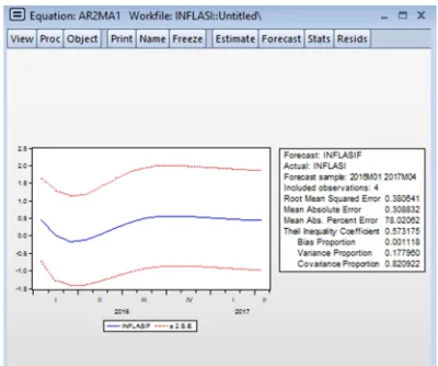
Figure 12. The Results Of The Estimation Model Of ARIMA(2,0,1) Or ARMA(2,1)

Based on the Figure 12 note that the value of the Bias Proportion Variance Proportion, and relatively small, and relatively higher Proportion Covariance,

which means that forecasting to be generated is said to be good, hence this model can predict further.

Based on the Figure 13 shows that inflation data forecast results in Semarang district in may 2016, i.e. 0.03, June 2016, i.e. 0.22, July 2016, i.e. 0.38, August 2016 0.49, i.e., September 2016, i.e. 0.55, October 2016, i.e. 0.56, in November 2016, i.e. 0.55, in December 2016, i.e. 0.52 October 2017 0.49, i.e., February, 2017, i.e. 0.47, March 2017, i.e. 0.45 and April 2017, i.e. 0.44.

Figure 13. Inflation Data Forecast Results In Semarang District

The results of the forecasting inflation at Semarang with model ARMA(2,1) or ARIMA(2,0,1) using Minitab software and Eviews in may 2016 – April 2017 is pretty stable. The highest inflation occurred in September, October, and November 2016. High inflation is happening likely due on the third month of the increase in price implied by the rise in the index in the Group spending such as food group, a food group so, drinking, smoking tobacco, group housing &, water, electricity, gas, fuel & group health, group education, recreation, sport group & transport, communications financial services & or index group clothing. Lowest inflation occurred in May and June 2016. Low inflation is happening likely due on both the month price decline shown by the decline in the index in the Group spending such as food group, a food group so, drinking, smoking tobacco, group housing &, water, electricity, gas, fuel & group health, group education, recreation, sport group & transport, communications financial services & or index group clothing.

According to Assistant II fields of Economy Development of Semarang Regency Setda

Dwinanta, A (2016) in

program 20th anniversary 495 Semarang and pioneered 2016 as part of the efforts of the local government in controlling the rate of inflation. Cheap means market where price sells Semarang Regency Government packages at bargain prices, especially to underprivileged citizens, so as to reduce their expenditure on everyday life. According to coordinating Minister for the economy in his Nasution, Darmin (1999) in www.bankjateng.co.id, the Government seeks to control prices of food commodities ahead of the fasting which fall at the beginning of June 2016. The Government's attempt to cause inflation in May and June 2016 becomes low.

Table 9. The Value Of The Inflation In May And June 2016 With Minitab, Eviews And Actual

Month /

Year Minitab Eviews Actual

May / 2016 -0,15 0,03 0,1

June / 2016 0,15 0,22 0,3

Based on Table 9 shows that the results of forecasting inflation at Semarang in May and June 2016 using Minitab software and Eviews, better approach with an actual value is to use software Eviews. This is because on software Eviews has a small forecasting errors and the accuracy of forecasting is good compared with the Minitab software only has a small forecasting errors only. This is shown with a small MSE value, Bias Proportion Variance Proportion and relatively smaller and relatively higher Proportion Covariance obtained on output software Eviews.

5. CONCLUSION

From the explanation above can be taken to the following conclusions:

(1) The right to ARIMA Model forecasting inflation at Semarang using Minitab software and Eviews is model ARMA(2,1) or ARIMA(2,0,1). The model ARMA(2,1) or ARIMA(2,0,1) is a better model when compared to the other models. This is indicated by the parameters in the model are already significant, the value of the SSE, MSE, AIC and the SBC that model which is smaller in compare to other models and already meets the test of independence. To foresee the next period of using model ARMA(2,1) or ARIMA(2,0,1) software with Minitab namely with the following equation:

= 1,3551 − 0,5756 + −

0,9789

and to foresee the next period of using model ARMA(2,1) or ARIMA(2,0,1) with software Eviews namely with the following equation:

= 1,3551 − 0,5756 + −

0,9789 .

(2) Results of forecasting inflation at Semarang district in may 2016 – April 2017 with methods ARIMA using Minitab and Eviews software is served by the following table.

Table 10. The Results Of The Forecasting Inflation At Semarang District With Methods ARIMA Using Minitab

Software

Table 11. The Results Of The Forecasting Inflation At Semarang District With Methods ARIMA Using Eviews

Software

Eviews has a small forecasting errors and the accuracy of forecasting is better than the Minitab, because MSE value of Eviews is smaller than the

Month Year Forecasting_Results

May 2016 -0,15

June 2016 0,15

July 2016 0,4

August 2016 0,55

September 2016 0,62

October 2016 0,62

November 2016 0,59

December 2016 0,54

January 2017 0,5

February 2017 0,47

March 2017 0,44

April 2017 0,44

Month Year Forecasting_Results

May 2016 0,03

June 2016 0,22

July 2016 0,38

August 2016 0,49

September 2016 0,55

October 2016 0,56

November 2016 0,55

December 2016 0,52

January 2017 0,49

February 2017 0,47

March 2017 0,45

Minitab, Bias Proportion Variance Proportion and relatively smaller and relatively higher Proportion Covariance obtained on output software Eviews.

Limitations of this study include: yet continued development and eviews Minitab macro program for the improvement of the accuracy of statistical and mathematical analysis. For further research, could be developed include: analyzing the accuracy of the statistical program packages in the case of other capabilities, analyze the macro program in such packages, developed a package of statistical programs to be more accurate in the calculation. REFFERENCES

[1]Akerlof, G., Dickens, W., and Perry, G., 1996,

The Macroeconomics of Low Inflation, Brookongs Paper on Economics Acrtivity, vol 1: 1-76

[2]Aswi & Sukarna. Time Series Analysis.Analisis. Theory and Application. Edited byMuhammad Arif Tiro. Makassar: Andira Publisher, 2006. [3]Ball,L. and Markiw, G., 1994b, Asymmetric

Price Adjusment and Economic Fluctuations,

Economic Journal, vol104(423):247-261

[4]Ball,L. and Markiw, G., 1995, Relative Price Changes as Aggregate Supply Shocks,

Quarterly Journal of Economics, vol 110(1): 161-193

[5]Berlian, Wilandari, Yuciana, & Yasin, Hasbi. Inflation forecasting by Group of Expenditure Food , Beverages , Cigarettes and Tobacco Use Variations Calendar Model (Case Study Inflation Semarang Indonesia) Gaussian Journal Statistics UNDIP, 3(4): 547 – 556.

Available in

http://ejournal-s1.undip.ac.id/index.php/gaussian (accessed March 29, 2016), 2014.

[6]BPS Semarang Indonesia. Official Statistics of Semarang : The development of the Consumer Price Index / Inflation in Semarang District Month April 2016. Available in http://semarangkab.bps.go.id/ website/ brs_ind/brsInd-20160502115416.pdf (accessed May 23, 2016), 2016.

[7]Brockwell, P.J.and Davis, R.A.(1991)Time Series: Theory and Methods, 2nd edn. New York: Springer-Verlag.

[8]Brockwell, P.J.and Davis,

R.A.(1996)Introduction to Time Series and Forecasting. New York: Springer-Verlag. [9]Dwinanta, A. Thrift So Efforts to Control

Inflation in Semarang regency . Available in http://jateng.tribunnews.com/2016/04/15/pasar-

murah-jadi-upaya-kendalikan-inflasi-di-kabupaten-semarang (accessed August 15, 2016), 2016.

[10]Dwitanto, Dimas Setyo.. Time Series Analysis for Predicting the Total Patient Treated in Blora Health Center Using Minitab Software 14. Semarang: FMIPA UNNES Publisher, 2011.

[11]Engle, Robert. GARCH 101: The Use of

ARCH/GARCH Models in Applied

Econometrics. Journal of Economics Perspective, 15(4): 157-1, 2001.

[12]Hadijah. Forecasting of Operational Reserve with Program Approach Using Minitab Arima. PT Surindo Andalan Publisher. Journal THE WINNERS, 14(1):13-19, 2013.

[13]Hendikawati, Putriaji. Forecasting Data Time Series : Methods and Applications with Minitab & Eviews. Semarang: FMIPA UNNES Publisher, 2015.

[14]http://www.bi.go.id/id/moneter/inflasi/pengenala n/Contents/Pentingnya.aspx (accessed March 29, 2016).

[15]Iriawan, Nur & Puji Astuti, Septin. Processing Data Statistics with Easy to Use Minitab 14. Yogyakarta: CV ANDI OFFSET Publisher, 2006.

[16]Makridakis, S, Wheelwright., S.C, & McGee V.E.. Forecasting Methods and Applications ( First Edition) . Translation by Untung Sus A & Abdul Basith . Jakarta : Erlangga publisher, 1995.

[17]Mishkin, Frederic S & Savastono, Miguel A.. Monetary Policy Strategis for Latin America.

Journal of Development Economics,

Forthcoming: 1-6, 2001.

[18]Muhson,A., 1999, Faktor-faktor yang Mempengaruhi Inflasi di Indonesia. Laporan penelitian DIK FIS UNY

[19]Nasution, Darmin. Summary Economy Update 2 Juni 2016. Available in http://bankjateng.co.id/content.php?query=new s&kat=content&id_content=1000 (accessed August 15, 2016}, 2016.

[20]Pindyck, R.S. & Rubinfeld, D.L..Econometric Models and Economic Forecasts. 3rd edition. McGraw-Hill, 1991.

[21]Puthong, Iskandar. Introduction to Micro and Macro Economics. Jakarta: Ghalia Indonesia Publisher, 2002.

[22]Santoso, Singgih Buisness Forecasting .Method of Today's Business Forecasting with Minitab and SPSS. Jakarta: PT.Elex Media Komputindo Publisher, 2009.

[24]Spiegel, M. R., Stephens, L. J. Schaum’s Outliers of Theory Problems of Statistics (3rdEdition). Translation by Kastawan, W & Harmein, I. Jakarta: Erlangga Publisher , 2007. [25]Subagyo, Pangestu . Forecasting concepts

and applications. Yogyakarta: BPFE Publisher, 1986.

[26]Sukirno, Sadono. Microeconomic Introduction Theory (3rd Edition). Jakarta: Rajawali Pers Publisher, 2008.

[27]Sunariyah . Knowledge of Capital Market (5th Edition). Yogyakarta: UPP STIM YKPN, 2006.

[28]Supranto. Statistical theory and applications.. Jakarta: Erlangga Publisher, 2001.

[29]Tandelilin, Eduardus. Portfolio and Investment Theory and Applications ( first Edition). Yogyakarta: Kanisius Publisher, 2010.

[30]Winarno, Wing Wahyu. Analysis

Econometrics and Statistics with Eviews (3rd Edition). Yogyakarta: UPP STIM YKPN Publisher, 2011.

[31]Ikrima TN and Harjum Muharam. Co-Integration And Contagion Effect Between Stock Sharia Market In Indonesia, Malaysia, Europe, America And When The Occurrence Greek Crisis. Jurnal Dinamika Manajemen. Universitas Diponegoro, Semarang, Indonesia. JDM Vol. 5, No. 2, 2014, pp: 131-146

[32]Rokhaniyah and Muh Rudi Nugroho. Analysis of Flypaper Effect on The City and Country Government Expenditures in Indonesia 2012-2014.Fokus Ekonomi(FE), Agustus 2015,

p. 100 – 113Vol. 10, No. 2 ISSN: 1412-3851. [33]Syahnur TA . Analysis of Effects of Inflation, Economic Growth and Investment Against Unemployment in Central Java Province. Essay. Department of Economic Development. Faculty of Economics. Semarang State University

[34]Waryanto B and and Yuan Astika Millafati. The Transformation of Ordinal Data to Interval Data Using Macros Minitab. Pusat Data dan Informasi Pertanian Informatika Pertanian