SMOKE DETECTION BASED ON IMAGE PROCESSING BY USING GREY AND TRANSPARENCY FEATURES

7227

FUZZY RULE INTERPOLATION METHODS AND FRI

TOOLBOX

1_{MAEN ALZUBI,} 2_{ZSOLT CSABA JOHANYÁK,} 3_{SZILVESZTER KOVÁCS,}

1, 3 _{Department of Information Technology, University of Miskolc, H-3515 Miskolc, Hungary}

2_{Department of Information Technology, John Von Neumann University, Hungary}

E-mail: 1_{[email protected],}2_{[email protected]}

_,

[email protected]

ABSTRACT

FRI methods are less popular in the practical application domain. One possible reason is the missing common framework. There are many FRI methods developed independently, having different interpolation concepts and features. One trial for setting up a common FRI framework was the MATLAB FRI Toolbox, developed by Johanyák et. al. in 2006. The goals of this paper are divided as follows: firstly, to present a brief introduction of the FRI methods. Secondly, to introduce a brief description of the refreshed and extended version of the original FRI Toolbox. And thirdly, to use different unified numerical benchmark examples to evaluate and analyze the Fuzzy Rule Interpolation Techniques (FRI) (KH, KH Stabilized, MACI, IMUL, CRF, VKK, GM, FRIPOC, LESFRI, and SCALEMOVE), that will be classified and comparedbased on different features by following the abnormality and linearity conditions [15].

Keywords: Fuzzy Rule Interpolation, Fuzzy Interpolating Function, FRI Toolbox, Sparse Fuzzy Rule Base, Missing Fuzzy Rules

1. INTRODUCTION

Former popularity of fuzzy control application was derived from the simple human-readable knowledge representation of fuzzy rules and the simple heuristic way of the control surface definition. Using fuzzy sets as linguistic terms and defining a control surface by fuzzy rules as overlapping fuzzy points was a simple way to express and implement a heuristic control strategy.

On the other hand, the heuristic definition of the fuzzy rule base in a higher dimensional problem is a challenging task. The traditional fuzzy systems, [1], [2] were implemented based on defining a complete rule base. In the complete fuzzy rule base, we have to consider all the possible rule base. The fuzzy reasoning is based on rule firing strengths i.e. rule matching calculated from the t-norm of fuzzy sets, the required rule base size is exponential with the number of the input dimensions.

However, in case the complete fuzzy rule base cannot be obtained for any reason (e.g. lack of expert knowledge base or no overlapping of fuzzy sets), then the classical reasoning methods cannot offer the desired conclusion. That happens because there may be a new observation that is not covered

directly by any of the current fuzzy rule base. In this case, the fuzzy rules are considered as a sparse rule-base. There are several application areas such as control system, intrusion detection system and etc., requested a conclusion for each observation. This case the classical reasoning methods could face the problem of missing conclusion for some of the observations.

Alternative fuzzy reasoning solutions, i.e. Fuzzy Rule Interpolation (FRI) methods can release the need for the complete rule-base by replacing the rule matching reasoning concept with fuzzy interpolating function. The Fuzzy Rule Interpolation (FRI) methods were produced to handle the case of sparse rule-base. FRI methods are suitable to produce a conclusion even if some observations are not covered directly by the fuzzy rules. Therefore, using the FRI methods there is no need to have a complete fuzzy rules. The most significant fuzzy rules are enough to generate the desired conclusion.

7228 unified numerical benchmark examples to evaluate and analyze of the Fuzzy Rule Interpolation Techniques (FRI) (KH, KH Stabilized, MACI, IMUL, CRF, VKK, GM, FRIPOC, LESFRI, and SCALEMOVE) that will be classified and compared based on the abnormality and linearity conditions.

The rest of the paper is organized as follows: Section (2) provides a brief review of the basic definitions of the classical reasoning and interpolative reasoning methods. Section (3) introduces an overview about enumeration of some of the implemented FRI methods. Description of the renewed and extended version of the original FRI toolbox is presented in section (4) and a set of some numerical examples of implemented FRI methods are presented in section (5). FRI methods results are discussed in section (6). Finally, section (7) concludes the paper.

2. PRELIMINARIES

This section provides a brief overview of the basic definitions of the complete fuzzy rule base and sparse rules. It also briefly introduces the description of the interpolative reasoning concept.

2.1 Complete and Incomplete Rule Bases Let us take into consideration two numerical variables X and Y described on the universe R of real numbers, and F is a set in the fuzzy sets of R. We assume the fuzzy sets Ai in F are defined, 1 ≤ i

≤ n, such that: A1  A2... Ai  Ai+1... An, for a

given order  on F. We also suppose that we are

given fuzzy sets Bi in F, 1 ≤ i ≤ n, which are also

ordered according to .

According to the definitions in [12], [13], the fuzzy functions are described by the fuzzy relations between the fuzzy sets of the inputs Ai and outputs

Bi. The fuzzy rule base could be characterized and

represented based on this relation. The classical reasoning methods, such as Mamdani and Sugeno [1], [2] follow that relation which require to define all the fuzzy rule base relations between the inputs and outputs, in addition, to define the overlapping between them to get the desired conclusion. Figure (1) describes the complete fuzzy rule base between two dimensions antecedents and single consequent, the observations (x1) and (x2) are matching with the fuzzy rules 1,2,4 and 5, thus, the conclusion could be computed based on one of the classical fuzzy reasoning methods, like the Zadeh-Mamdani max-min Compositional Rule of Inference (CRI).

Figure 1: Complete Fuzzy Rule Base

Regarding the sparse base (incomplete rule-bases) systems where fuzzy rules are of the type: (Ri): “if X is Ai then Y is Bi”. The sparsity means there is no overlapping between the observation and any of the fuzzy rules (do not cover the input space F), where there exist inputs A∗ _{such that ∃i / Ai }

A∗ _{ Ai+1. The aim of a fuzzy interpolation method}

is to provide the conclusion corresponding to the observation A∗ _{by considering only the two rules Ri}

and Ri+1 when Ai  A∗ _{ Ai+1.}

Figure (2) describes the issue, where the observations x1.1 and x1.2 refer to the first input

(antecedent 1), the observations x2.1 and x2.2 refer to

the second input (antecedent 2). These observations are described two different types of issues in classical reasoning. The observations x1.1 and x2.1

are not overlapped with any of the rules of the rule-base, while, the observations x1.2 and x2.2 hit spaces

in the universe of discourse, there are no linguistic terms defined, hence no overlapping rule can exist.

7229 2.2 Notation of FRI

According to the definition of the fuzzy function, the fuzzy space can be described by the mapping between antecedents and consequents fuzzy sets LX _{and L}Y _{via f: L}X _{→ L}Y_{. This leads to}

the main idea of the fuzzy rule interpolation methods which is finding a suitable fuzzy interpolating function.

These functions could be able to produce a conclusion directly even if the rule base is sparse, and there is no overlapping between the observation and any of the fuzzy rules.

Many of the fuzzy rule interpolation (FRI) methods following the notion in [3], [14], [15] which describe the relation between two fuzzy rule base, these fuzzy sets must be adjacent convex and normal (CNF) and partially ordered fuzzy sets. Where the ordering is defined as A1, is said to be

“less than” A2, for all A1, A2 sets in a given fuzzy

partition. the ordering of the fuzzy set A1 and A2,

denoted by A1 ≺ A2, if α[0,l], the following

condition hold:

inf(A1α) < inf(A2α), sup(A1α) < sup(A2α),

Where the "inf" denotes the infimum and "sup" refers the supremum of the (A1α), (A2α) fuzzy sets.

For simplicity, suppose that two fuzzy rules are given:

If X is A1 then Y is B1

If X is A2 then Y is B2

Where the fuzzy rules are described by A1⇒ B1

and A2⇒ B2. Also, that rules in a given rule base

are arranged with respect to a partial ordering among the convex and normal fuzzy sets (CNF sets) of the antecedents, consequent and observation. For the above two rules, this

means

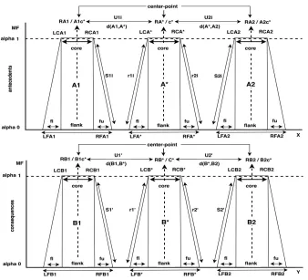
A1≺ A∗≺ A2 ∧ B1≺ B2

Figure (3) illustrates the simplest form to describe two flanking rules of the fuzzy sets, where the shape of the fuzzy sets membership functions remained restricted to trapezoidal, the figure shows the main points (variables) of the fuzzy sets to be applied for determining the conclusion in most FRI methods.

7230 Where A1, A2 refer to the fuzzy sets of the

antecedents, B1, B2 denote the consequent fuzzy

sets. A∗ _{denotes to the new input (observation), B}∗

refers to the conclusion. The characteristic points of the trapezoidal membership function could be defined by four values (LF, LC, RC, RF), the (LC, RC) refer to the left and the right core, the (LF, RF) refer the left and the right flank. (RA1, RA∗, RA2)

denote the center point of the fuzzy sets in antecedents side and similarly the (RB1, RB∗, RB2)

denote the center points of the fuzzy sets in consequents side, (fl, s2, r1) and (fu s1, r2) denote the left and the right fuzziness for each fuzzy set, (Ui, U’) denotes the distance between the center points of the fuzzy sets.

3. FRI METHODS

There are many fuzzy rule interpolation methods exists, classified into two groups. The first group obtains the conclusion in a single step (directly) and the second group demands two-steps to compute the conclusion, using different algorithms in each step. This section presents an overview about some of the implemented FRI methods.

3.1 KH Interpolation Method

The first method which was proposed for FRI is called the KH (linear interpolation) method, this method was published by Kóczy and Hirota [3]. Concerning the common general conditions for FRI methods suggested in [15], The KH rule interpolation method needs the following conditions to be satisfied: the fuzzy sets in both antecedents and consequents must be convex and normal (CNF) with bounded support and at least a partial ordering must exist between fuzzy sets in the universes of discourse.

The conclusion in KH interpolation method produced directly based on the α-cuts of the observation and the fuzzy rule-base, it can be calculated by using the fundamental equation of the KH FRI (1), which is based on the lower and upper fuzzy distances between fuzzy sets [16]. The upper and lower endpoints could be used to calculate the distance between the conclusion and the consequent which must be analogous to the upper and lower fuzzy distances between observation and antecedents.

d(A*, A1):d(A*, A2) = d(B∗, B1):d(B∗, B2) (1)

Where (d) refers to the Euclidean distance that could be used between the fuzzy sets (A1, A2) and

(B1, B2).

The conclusion B∗ _{in this method could be}

calculated based on the lower and upper fuzzy distances between the fuzzy sets of the antecedents, consequent and observation. Figure (3) illustrates the main points (core and flank) of the trapezoidal fuzzy sets which could use in order to compute the conclusion B∗ _{as follows:}

The right (core) can be calculated by the Equation (2):

RCB* ₌

RC

d

RC

d

RCB

RC

d

RCB

RC

d









1



   k i i i RCA RCA RC d 2 1 * 2

2



   k i i i RCA RCA RC d

And the right (flank) can be calculated by Equation (3):

RF

d

RF

d

RFB

RF

d

RFB

RF

d

RFB











1



   k i i i RFA RFA RF d 2 1 * 2

2



   k i i i RFA RFA RF d

The left (core) and the (flank) can be obtained similarly to the above Equation (2 and 3).

7231 3.2 The KH Stabilized Method

Many studies introduced a modification of the original KH method to improve the abnormality and to take more than two rules throughout the determination of the conclusion, the extended method was developed to handle and decrease the abnormality of the original KH method is called KH Stabilized that was proposed by Tikk, .et.al. [5].

The main idea of this method is to take all flaking rules of the observation which is getting better with the growth of the number of the rules taken into consideration to conclude the conclusion, using the extent of the inverse distance of the antecedents and observation of fuzzy sets. The universal approximation property holds if the distance function is raised to the power of the inputs dimension.

The authors of [5] propose using formulas to calculate the upper and lower endpoints of α- cuts of the approximated consequence which contain the distance on the nth _{power as shown via the}

Equations (4 and 5):









The simplest of the KH Stabilized method is the linear interpolation of two rule-bases for the area between their antecedents. In addition, this method can be applied if the observation position is located between two closest rules or hits outside rule-bases.

3.3 VKK Interpolation Method

This method was proposed by Vas, Kalmar and Kóczy [4]. The main idea of this method is based on the center point and width ratio, the conclusion could be calculated by the center point and width

ratio between the antecedent, consequent, and

observation fuzzy sets.

The center point of the conclusion can be

obtained by Equations (6, 7 and 8):

) , ( ) ( 2 *   i il A A d r RightCente LeftCenter B

Center   (6)

) ( )

,

( * _{2 1}

 

 Ai Center Bi

A d

LeftCenter   (7)

) ( )

,

( * ₂

1  i  i A Center B

A d

RighCenter   (8)

Where 2 ) sup( ) inf( ) (  

 A A

A

Center  

The width ratio of the conclusion can be

calculated by Equations (9, 10 and 11):

* 2 1 * ) , ( ) ( WA A A d RightWidth LfetWidth B Width i i      (9) ) / ( ) ,

(A* Ai2 Width Bi1 WA1i d

LeftWidth      (10)

) / ( ) ,

( 2 2

*

1 i i

i A Width B WA

A d

RightWidth  _{ }  _ (11)

Where

)

inf(

)

sup(

)

(

A

A

A

Width





The d(Ai1α, A∗α), d(A∗α, Ai2α) and d(Ai1α, Ai2α))

refer to the distance between antecedents fuzzy sets, the geometric average of the width values metrical is represented by (WA1i), (WA2i), and (WA∗)

between the antecedents and observation.

The disadvantage of this method is the abnormality can be appeared in some cases. Nevertheless, the VKK method is distinguished by a low complexity compared to the KH method due to the calculation of the conclusion directly through the center and the width of the fuzzy sets. It is also simple and can be used in several applications without complications.

3.4 MACI Interpolation Method

Another method of the FRI called the Modified α-Cut based Interpolation (MACI) method was proposed by Tikk and Baranyi [6]. The main idea of this method is based on the vector’s description of the fuzzy sets for eliminating the abnormality problem in the conclusion. The fuzzy set in this method could be described by two vectors space, it can represent the Left and the Right flank of the α-cut levels where the abnormal consequent set is excluded.

The characteristic points that are used in vector description can be represented by the piecewise linear shape of the fuzzy sets where (a−1, a0)

describe the left flank, and (a0, a2) represent the

7232 the fuzzy set, the Cartesian axes can be represented by Z0, Z1 as shown in Figure (4).

Figure 4: The Vectors Description Input And Output Fuzzy Sets [6].

The conclusion in this method could be determined by the transformation of the current characteristic points to a new Cartesian to calculate the conclusion, then, transforming back to the original Cartesian to show the result that could be computed by using the following Equations (12, 13 and 14):

The new Cartesian can be calculated by the vector form:

b = [

b

b

b

b

b

' 0

b

b

2

b

b

b

The vector description can be represented by the matrix:

b’ = bT (14) Where

T =

_













1

1

0

2

The MACI method concentrates on the characteristic points of the fuzzy set (A1, A∗ and A2)

and the consequents (B1 and B2). It can be described

by vectors which involve computing the center point of the conclusion RB∗ _{as shown in Figure (3).}

The conclusion could be calculated by Equation (15) as follows:

RB*_=(1-



core)RB1 +



Where





 







k

i i i k

i i i core

RA

RA

RA

RA

1

2 1 2

2

1 1

*

)

(

)

(



Where, the RA∗_{, RA1, and RA2 denote the}

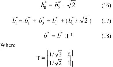
reference point of the observation and antecedents fuzzy sets. After computing the conclusion could be transformed back to the original Cartesian by the vector form by applying the Equations (16, 17 and 18):

* 0

b

b

2

* 1

b

b

b

b

b

2

*

b

b

Where

T =

    

  

1 2 / 1

0 2 / 1

For more detailed description of MACI function can be found in [19], [20].

The main advantage of the MACI method is that the conclusion is always a convex and normal fuzzy set. It can also apply multi-dimensional antecedents [6]. On the other hand, the disadvantage of this method (in some instances) is that it does not keep the piecewise linearity of the membership functions.

3.5 CRF Interpolation Method

This method was proposed to modify the fuzziness term and to improve α-cut levels. The main idea of this method was introduced in [21] which was called GK method, also the modified version of the GK called the KHG method was published by Kóczy, Hirota, and Gedeon in [7]. The current modified version is called the conservation relative fuzziness (CRF) which follows fundamental equation (FEFRI) (1). This method aims to obtain the conclusion based on determining the core and fuzziness of antecedents, consequents and observation fuzzy sets, the core c∗ _{could be}

described by (A1c∗, A2c∗, A∗c∗) and (B1c∗, B2c∗) as

shown in Figure (3), the core of the conclusion could be calculated by using the distances between the antecedents and observation as d(A∗, A1) and

d(A2, A∗), also between the consequents fuzzy sets

7233 In addition, the fuzziness of the conclusion could be determined by calculating the (A1fU,

A∗_{fL) that must have the same fuzziness of the}

(B1fU, B∗fL), and similarly the fuzziness between

(A∗_{fU, A2fL) and (B}∗_{fU, B2fL) as shown in Figure}

(3).

The core of the conclusion C∗ _{can be calculated}

by Equation (19):

)

,

(

)

,

(

*

A

A

d

B

B

d

c

C





Where c∗ denotes the core of the observation, and d1 denotes the distance between A1 and A2

which can be calculated as follows:

d1=(A1,A2) = A2c* - A1c*

d1=(B1,B2) = B2c* - B1c*

The general fundamental Equation (1) can be applied to determine the distance between the current fuzzy sets through Equation (20):

)

,

(

)

,

(

)

,

(

)

,

(

B

B

d

B

B

d

A

A

d

A

A

d

_

So, Equation (20) can be used to calculate the core of the conclusion by the distance of the following Equation (21 and 22):

)

,

(

)

,

(

)

,

(

)

,

(

A

A

d

B

B

d

A

A

d

B

B

d





And similarity,

)

,

(

)

,

(

)

,

(

)

,

(

A

A

d

B

B

d

A

A

d

B

B

d





Where the distance between the fuzzy sets can be computed as the following formula:

2 2 * 1 * 2 2 1 1

)

(

)

,

(

range

A

A

A

A

d

_



The fuzziness of the conclusion can be determined by the left and the right flanks by the current fuzzy sets as follows by Equations (23 and 24): fU fU fL fL

_A

B

A

B

*

_

_

fL fL fU fU

_A

B

A

B

*

_

_

Accordingly, the equations in [7], it is possible to compute the A∗_{fL, A}∗_{fU, A1fU, A2fL, B1fU, and}

B2fL which are based on the calculation of the (inf)

and (sup) of the current fuzzy sets.

The previous Equations (19-24) of the CRF method were introduced to be applied by single dimensional input, and also, it can be applied in multi-dimensional input by using the expression in [7].

The advantage of this method is that the flanks are used to define the conclusion, therefore, this method can be applied arbitrarily on fuzzy set shapes. Additionally, the observation position must be surrounding two rule-bases s to get a conclusion.

3.6 IMUL Interpolation Method

This method was proposed by Wong, Gedeon and Tikk [8], the IMUL is introduced to avoid the abnormal conclusion and improve the multidimensional α-cut (levels). This method was presented to combine the features of MACI method [6] and Conservation of Relative Fuzziness (CRF) method [7].

The IMUL method applied the vector description, it can describe the characteristics points of the fuzzy sets through advantageous the transformation feature of MACI method, and representing the fuzziness of the input and output by CRF method. The conclusion could be calculated between the characteristic points of the antecedent fuzzy sets which are neighboring to the observation as shown in Figures (3).

The conclusion in IMUL method is based on calculating the reference point (RB∗_{) and the left /}

right core (LCB∗_{, RCB}∗_{), the reference point could}

be computed by Equation (8). The left and right core can be calculated through the following Equations (25 and 26):

The right core:

RCB*_{= (1-}



right)RCB1 +



RCB2+ (





7234 where





 







k

i i i k

i i i right

RCA

RCA

RCA

RCA

1

2 1 2

2

1 1

*

)

(

)

(



The left core:

LCB*_{= (1-}



left)LCB1 +



(





where





 







k

i i i

k

i i i left

LCA

LCA

LCA

LCA

1

2 1 2

2

1 1

*

)

(

)

(



The conclusion flanks (LFB∗_{, RFB}∗_{) can be}

computed by following Equation (27):

The left flank:

)

'

'

1

(

* *

U

S

U

S

r

LCB

LFB









Where the LFB∗ _{denotes the left flank fuzziness}

of the conclusion B∗_{, and the LCB}∗_{denotes the left}

core, the right flank can be calculated in the same way, the variables (r, s, u, s’, u’) are used to determine the fuzziness between the fuzzy sets to calculate the conclusion flank ([8], [19]).

One of the benefits of using IMUL method is that the conclusion can be obtained by computing core and fuzziness focusing on the information of the consequents (outputs) and the information of the antecedents fuzzy sets that are given correct results. Moreover, IMUL method can be applied on single dimension and also in multi-dimensional inputs space (see the examples in [8]).

3.7 GM Interpolation Method

The first method in the second group of the interpolation methods which demanded two-steps to get the conclusion is called GM method. It was published by Baranyi et al. [9], the conclusion in this method could be determined by two algorithms. The first one is based on the fuzzy relation and the second one is based on semantics of the relations. The GM method will adopt the characterization of the position fuzzy sets to determine the reference points (core), thus, the distance between the observation and antecedents fuzzy sets can be calculated based on the reference points via

Equation (28) instead of using the interpolating α-cut levels.

d(A1,A2) = | RP(A2) – RP(A1) | (28)

where A1 and A2 are the fuzzy sets, the

reference point is (RP) and (d) denotes the distance of the sets.

The conclusion (interpolation) can be obtained by applying the following primary two steps:

The first step is to generate a new interpolated rule Ri_{: A}i _{→ B}i_{, which is positioned between rules}

R1 and R2 via Equation (29), the position of the new

rule is the same position of the observation, so, each fuzzy set of the antecedents is used to produce the new rule which must be identical with the reference point of the observation fuzzy set in the corresponding dimension.

)

,

(

R

R

f

R

_

This step could be divided into three stages: 1. The first stage, a set interpolation technique

will help to determine the antecedent set shapes of the interpolated rule.

2. The second stage, the reference points of the observation and the consequent sets can be used to determine the reference point of the conclusion, where the rules could be taken into consideration, for example, using the fundamental equation of the fuzzy rule interpolation (FEFRI) (Equation (1)). 3. The third stage, the shapes of the consequent

sets could be determined by the interpolated rule using the same set interpolation technique as (stage 1) as shown in Figure (5).

Many techniques were proposed for this step of the set interpolation technique (e.g. SCM, FPL, etc.). The Solid Cutting Technique (SCM) is introduced for this step, the main idea of this technique is that all the associated sets are rotated by 90° _{about a vertical axis which is passed through}

7235 Figure 5: The Main Steps Of The GM Method [9].

The second step in the GM method is that the new rule could be specified as a part of the extended rule of the approximate conclusion, as a conclusion of the inference method is defined by determining this rule. In many instances, there is no identical similarity between the rule and the observation part, for this purpose, many techniques are used to handle the mismatch by either the Transformation of the Fuzzy Relation (TFR) technique or by Fixed Point Law (FPL).

This step could be divided to two stages:

The first stage, the Transformation of the Fuzzy Relation (TFR) technique could be applied, where the interrelation function [9] is generated between the observation (A∗_{) and the antecedent (A}i_{) set,}

there is mapping between observation (A∗_{) and}

antecedent (Ai_{) by the endpoints of the support and}

reference point (RP), as shown in Figure (6), the interrelation area can be represented by the endpoints of the supports sets. The purpose of the first phase is to improve the proportion of the area of interrelation mapping between (Ai _{and B}i_{) sets, it}

can correspond with the support of the observation and the horizontal side of the square. Hence, the support of the conversion set (At_{) is the same}

support of the (A∗_{), the membership in both cases}

(At, A∗_{) is the same as its interrelated point in the}

Antecedents part.

Figure 6: The Interrelation Functions [9].

The second stage, the FPL (Fixed Point Law) technique can be used where an interrelation function is created between observation (A∗_{) and}

the transformed antecedents sets (At_{), the (FPL)}

technique is used to calculate the difference between the membership values for each interrelated point set, this difference can be applied to determine the approximate conclusion from the transformed consequent sets (Bt_{) that will take into}

consideration the interrelation between transformed (At_{) and transformed (B}t_{) [9].}

The main advantage of this method (GM) is to avoid the abnormal fuzzy conclusion, there is no restriction to CNF sets and preserving normality, it preserves linearity and is compatible with the rule base, finally it investigates the monotonicity and the continuity.

3.8 FRIPOC Interpolation Method

A new fuzzy interpolation method which is based on the reasoning method by using the concept of the linguistic term shifting and polar cut which is called Fuzzy Rule Interpolation based on POlar Cuts (FRIPOC), this method was proposed by Johanyák and Kovács [10], where it is appropriate in case of sparse and dense rule bases. The general formula that can be described to show the reference point which is specified to calculate the interpolated of the Antecedents RP(Ai

j) and the consequent

RP(Bi

l) sets which could be calculated by Equation

(30).

) ), ( ),.., ( ),.., ( ), (

( 2

i na i

j i

i l i

l f RP A RP A RP A RP A

RPB  ₍₃₀₎

This method is based on the position of the fuzzy sets which is characterized by a reference point during the calculations, the reference point RP(Bi

l) can be determined by several techniques

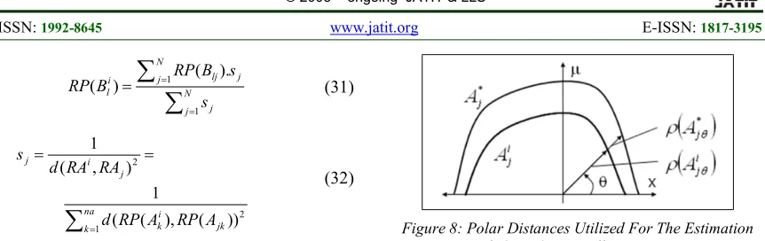
Figure (7). The presented technique to determine the reference point can be calculated by Equations (31 and 32). The FRIPOC method essentially follows the GM method [9], where the conclusion can be done by applying two steps: the first step is to define the new rule based on the position of the antecedents part that describes the observation in each dimension, this means the reference point of the observation and antecedents set are identical.

7236





j lj j

i l s s B RP B RP 1 1 ( ).

) ( (31)   ₂ ) , ( 1 j i j RA RA d s (32)



k RP A

A RP d 1 2 )) ( ), ( ( 1

Where RP(Bi

l) is the RP of the consequent sets,

sj denotes to weight attached to the rule, (l) refers to

the number of dimensions, (N) denotes the number of the rules, (j) refers to the actual rule, RAi _and

RAj denote the antecedent rule [10].

Accordingly, the new rule could be determined by two steps: The first step could be described by three stages as follows: 1) the fuzzy sets of the antecedents are estimated by utilizing the set interpolation technique Fuzzy SEt interpolAtion Technique bases on Polar cut (FEAT-p) that is independently in each antecedent dimension, the main purpose of this technique is that the whole sets of the partition are shifted horizontally into the reference point of the observation, i.e. their reference points are identical with the interpolation point. 2) the new fuzzy set is determined based on the polar cut, where the fuzzy set can be specified by using the polar distance of each polar cut level as a weighted mean of the similar polar distances of the forecasted identified sets. 3) the fuzzy set will determine the consequent by FEAT-p technique in the same way as (first stage). Thus, the new fuzzy set can be calculated by following the formula as shown in Equation (33).

             



_

The second step in FRIPOC method defines the conclusion which is generated by exciting the new rule based on using the Single Rule Reasoning based on polar cuts (SURE-p) technique [10]. The reference point of the interpolated conclusion and the consequent set are identical to the new rule in the current dimension. Figure (8) describes the distance of the polar that can be calculated based on each polar level, the conclusion can be computed by the modified consequents of the interpolated rule using the average differences, where the technique of correction and control could be used to guarantee the efficacy of the new fuzzy set.

Figure 8: Polar Distances Utilized For The Estimation Of The Relative Difference [11].

The main benefits of the FRIPOC method are comprehensibility, the ability to applicability in subnormal cases, and also can be applied if there are no rules surrounding of the observation (extrapolation).

3.9 LESFRI Interpolation Method

This method follows the GM method by computing the conclusion based on two steps, this method is called LEast Squares based Fuzzy Rule Interpolation (LESFRI) and was proposed by Johanyák and Kovács Szilveszter [11].

The main idea of this method is the conservation of the weighted average differences measured on the antecedent part, where these modifications could be applied on the consequent side, in which the results usually could be as a set of characteristic points that will not fit with the default shape type of the partition. Therefore, the LESFRI method could be used in order to find the breakpoints of an adequate conclusion. The LESFRI method is based on two-step:

The first step aims to define the interpolation point of the new fuzzy set which can be achieved by three stages as follows [11]:

1. The FEAT-LS technique is used to calculate the antecedent sets for each dimension, where this technique aims to generate a new fuzzy set based on the interpolation points of the fuzzy partitions, thus, all the sets of the partition are shifted horizontally in order to reach the coincidence between their reference points and the interpolation point by using Equation (34).



j w X X

7237 2. The position of the consequent fuzzy sets can

be determined for each consequent dimension of the new rule by utilizing a crisp interpolation method by Equation (35).



 ₂

) , (

1

j i l

RA RA d s

(35)



na

k lj

i

j RP A

A RP d

1

2

)) ( ), ( (

1

3. The characteristic points of the new fuzzy sets shapes are defined by the method of weighted least squares by taking into consideration the similar characteristic points of the overlapped sets which could be used to estimate the conclusion using the observation and the new rule.

The second step in the LESFRI method is the conclusion that could be produced based on the new rule which is required for the calculation of the conclusion because the points of the rule do not fit ideally with the observation in each input dimension. The method that was proposed for this purpose is called SURE-LS as a single rule reasoning method which is based on the α-cut approach. Consequently, all the current antecedent dimensions and consequent fuzzy sets could be described by the break-point α-levels to calculate the conclusion, it must be done independently to the left and right flanks of the fuzzy sets. Additionally, the weighted average of the distances between the endpoints the α-cuts of the rule antecedent and the observation set could be calculated to each side for each level.

The advantages of this method are its capability to produce new linguistic terms that fit into the regularity of the original partitions, as well as its low computational complexity, where it can be applied in case of the interpolation and extrapolation.

3.10 Scale and Move Interpolation Method The scale and move transformation-based method was produced by Huang and Shen [22], it follows the interpolation concept to handle the sparse fuzzy rules. The scale and move method provides the capabilities to work with different fuzzy membership functions types such as (Triangular, Trapezoidal).

The scale and move method is based on the Centre Of Gravity (COG) of the membership

functions as shown in Figure (9), this method based on generates a new central rule-base via two neighboring rule-bases that are surrounding the observation.

Figure 9: Representative Value Of A Triangular And Trapezoid Fuzzy Sets [22].

This scale and move method follows two-steps to obtain the conclusion, the first step is to produce a new central rule-base (A` → B`) is produced within the existing surrounding rule-bases between observation (A∗_{: A1 → B1, A2 → B2) through to}

apply the Equation (36):

))

(

),

(

(

))

(

),

(

(

2 1

* 1

A

REP

A

REP

d

A

REP

A

REP

d

REP





Where d(Rep(A1); Rep(A2)) represents the

distance between two fuzzy sets A1 and A2. Rep(A1)

refer to the center of gravity for A1 [22].

The new rule-base (A` → B`) can be calculated by Equations (37 and 38):

2 1

)

1

(

'

A

A

A











20 10

,

0

(

1

)

a

a

a











21 11

,

1

(

1

)

a

a

a











22 12

,

2

(

1

)

a

a

a











2 1

)

1

(

'

B

B

B











20 10

,

0

(

1

)

b

b

b











21 11

,

1

(

1

)

b

b

b











22 12

,

2

(

1

)

b

b

b











The degree of similarity between A` and A∗ _is

set, it is natural to require that the consequent part B` and B∗ achieve the same similarity degree as follows:

7238 Therefore, the second step is to calculate the A` similarity degree between fuzzy sets (A` and A∗) that is to allow transforming B` to B∗ with the desired degree of similarity by the scale and move. The aim of the Scale transformation is to change the support value of the membership function while keeping its representative value and shape, the aim of the move transformation is to transfer the support of the membership function with keep of its representative.

The advantages of scale and move method that it can handle multiple antecedent variables with simple computation. It guarantees the normality and convexity of the conclusion fuzzy set. It offers the capability to handle the extrapolation issue in direct manner [23]. It preserves the piecewise linearity for interpolations involving arbitrary polygonal fuzzy sets and it uses various definitions for representative values.

4. GENERAL DESCRIPTION OF FRI

TOOLBOX

The FRI toolbox was developed by Z.C. Johanyák, .et. al. [24] and implemented in MATLAB environment. The main goal of the FRI toolbox is to unify different fuzzy interpolation methods. The general structure of FRI toolbox presented in Figure (10) can run the FRI toolbox and could be used to evaluate the current FRI methods.

Figure 10: The General Structure Of FRI Toolbox The current version of FRI toolbox is available to download in [26], it includes the following methods (KH, KH Stabilized, MACI, IMUL, CRF, VKK, GM, FRIPOC, LESFRI, and SCALE

MOVE). The package of FRI toolbox contains a software with graphical user interface providing an easy-to-use access as shown in Figure (11).

Figure 11: The Main Panel Of The FRI Toolbox [24]

In the FRI toolbox, the structure of the fuzzy inference system (FIS) and observation (OBS) were different from the classical inference system. Figure (12) presents an example of FIS within the FRI toolbox. It worths mentioning that, the fuzzy sets have to be convex and normal [3], [25].

Figure 12: The New Parameters Of The Membership Functions That Are Used By The File System In FRI

Toolbox

Where the (trimf), (trapmf) and (singlmf) denote the triangular, trapezoidal and singleton shapes of the fuzzy sets respectively. The A1;1, A2;1 and B1;1

refer to the names of the fuzzy sets of Antecedents and consequent parts. The values [10 20 30], [4.5 5 5.5 6] and [0.46] denote the characteristic points (params) of the fuzzy sets in the universe of the discourse, where the triangular shape takes three values [a0, a1, a2], the trapezoidal shape can be

represented by four values [a0, a1, a2, a3], and

singleton shape could be described by one value [a0].

7239 a1, a2, a3], where the points [a0, a3] refer to the level

(0) (lower level) and the points [a1, a2] refer to the

level (1) (upper level). Figure (12) describes the new parameter for the trapezoidal membership function (trapmf) which represented by [0 1 1 0].

5. NUMERICAL EXAMPLES

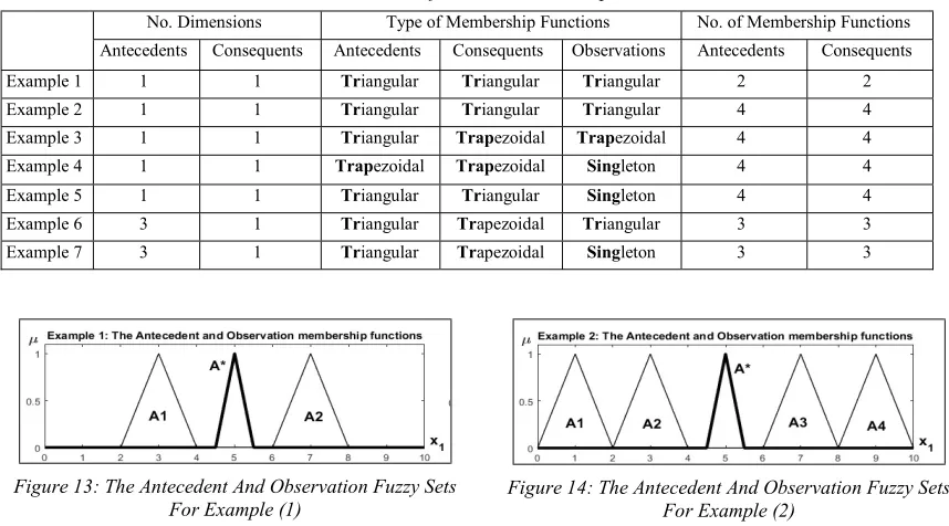
In this section, the following (FRI) methods (KH, KH Stabilized, MACI, IMUL, CRF, VKK, GM, FRIPOC, LESFRI, and SCALE MOVE) are presented and discussed in details. The unified numerical examples are applied for the sake of investigating and comparing the FRI methods. These examples selected based on various features, the number of dimensions, the shape of membership functions and the number of membership functions.

Results of these examples would be used to evaluate the FRI methods by following the general conditions of the fuzzy interpolation concept [15], the abnormality and linearity.

These examples were chosen to test the current FRI methods by using FRI toolbox. The triangular, trapezoidal and singleton membership functions are used to describe the antecedent, consequent and observation. Seven examples will be introduced in this section to test the current FRI methods.

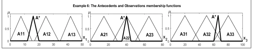
Figure 13: The Antecedent And Observation Fuzzy Sets For Example (1)

The first two examples, single dimension is described the antecedent and consequent, these examples will compare the results based on the difference between the number of the fuzzy sets by using the same membership functions for antecedent, consequent and observation.

The third example will represent the antecedent and consequent by a single dimension, the same number of the fuzzy sets is used for the antecedent, consequent part. This example describes the antecedent, consequent by a different membership function, where the observation represented by the trapezoidal membership function.

The fourth and fifth examples were selected to show the results by using the same membership functions of the antecedents and consequent using different shapes of the observation. These examples are described by using different dimensions, where the antecedent parts are represented by three dimensions and the consequent represented by single dimension.

Table.1 summarizes the unified numerical examples. The antecedents and observations are shown in Figures (13 to 19), the consequents part and conclusions have appeared in Figures (20 to 29).

Figure 14: The Antecedent And Observation Fuzzy Sets For Example (2)

Table 1: The Unified Numerical Examples.

No. Dimensions Type of Membership Functions No. of Membership Functions

Antecedents Consequents Antecedents Consequents Observations Antecedents Consequents

Example 1 1 1 Triangular Triangular Triangular 2 2

Example 2 1 1 Triangular Triangular Triangular 4 4

Example 3 1 1 Triangular Trapezoidal Trapezoidal 4 4

Example 4 1 1 Trapezoidal Trapezoidal Singleton 4 4

Example 5 1 1 Triangular Triangular Singleton 4 4

Example 6 3 1 Triangular Trapezoidal Triangular 3 3

7240 Figure 15: The Antecedent And Observation Fuzzy Sets

For Example (3)

Figure 20: Numerical Examples: KH Conclusions

Figure 16: The Antecedent And Observation Fuzzy Sets For Example (4)

Figure 21: Numerical Examples: KH Stabilized Conclusions

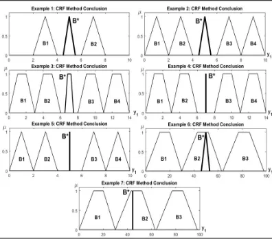
Figure 18: The Antecedents and Observations Fuzzy Sets for Example (6)

7241 Figure 22: Numerical Examples: MACI Conclusions

Figure 23: Numerical Examples: IMUL Conclusions

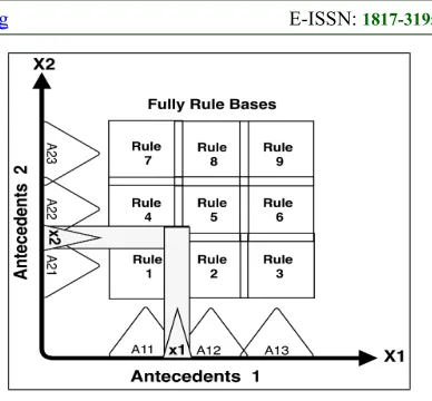
Figure 24: Numerical Examples: CRF Conclusions

Figure 25: Numerical Examples: VKK Conclusions

Figure 26: Numerical Examples: GM Conclusions

7242 Figure 28: Numerical Examples: LESFRI Conclusions

Figure 29: Numerical Examples: Scale and Move Conclusions

6. RESULTS AND DISCUSSION

The aforementioned results of the numerical examples conclude the following:

According to the antecedents and observations shown in Figures (13,14,16 and 17), the following methods (KH, KH Stabilized, MACI, IMUL, CRF, VKK, GM, FRIPOC, LESFRI, and SCALE MOVE) could be a suitable approach to be implemented as an inference system in a single dimension antecedent, the antecedent and consequent have the same type of membership functions (Triangular / Trapezoidal), despite the type of observation membership functions shown in Figures (20 to 29) which illustrated in examples (1,2,4, and 5).

With regard to the antecedents and observations shown in Figure (15), the following methods (KH, KH Stabilized) could be a suitable approach to be implemented as an inference system in a single dimension antecedent, the antecedent and consequent have different type of (Triangular and

Trapezoidal) respectively, based on the type of the

observation shown in Figures (20 and 21) which represented in examples (1,2,4, and 5).

According to the antecedents and observations shown in Figure (15), the following methods (MACI, IMUL, CRF, GM, FRIPOC and LESFRI) could be a suitable approach to be implemented as an inference system in a single dimension, the antecedent and consequent have different type of

(Triangular / Trapezoidal), regardless of the type of

the observation shown in Figures (22, 23, 24, 26, 27 and 28) which illustrated in example (3).

Regarding the antecedents and observations shown in Figures (18 and 19), the following methods (MACI and GM) could be a suitable approach to be implemented as an inference system in multi-dimension antecedents, the antecedent and consequent have different type of membership function (Triangular / Trapezoidal), despite the type of observation membership functions shown in Figures (22 and 26) which described in examples (6 and 7).

For antecedents and observations shown in Figures (18 and 19), the following methods (IMUL and CRF) could be a suitable approach to be implemented as an inference system in multi-dimension antecedents, the antecedent and consequent have different type of membership function (Triangular and Trapezoidal), regardless of the type of observation membership functions shown in Figures (23 and 24) which defined in examples (6 and 7).

Regarding the antecedents and observations shown in Figure (19), the following method (FRIPOC) could be a suitable approach to be implemented as an inference system in multi-dimension antecedents, the antecedent and consequent have different type of membership function (Triangular and Trapezoidal), in case of the type of observation membership function is singleton shown in Figure (27) and defined in example (7).

On the other hand, regarding the antecedents and observations shown in Figure (15), the following method (VKK) suffers from the abnormality in a single dimension antecedent, the antecedent and consequent have different type of

(Triangular and Trapezoidal) respectively, based

7243 Referring to the antecedents and observations shown in Figures (18 and 19), the following methods (KH, KH Stabilized and VKK) suffer from the abnormality in multi-dimension antecedents, whereas the antecedent and consequent have different type of membership function (Triangular /

Trapezoidal), regardless of the type of observation

membership functions shown in Figures (20, 21) and 25) which described in examples (6 and 7).

For to the antecedents and observations shown in Figure (18), the following method (FRIPOC) suffers from the piecewise linearity in multi-dimension antecedents, whereas the antecedent and consequent have different type of membership function (Triangular / Trapezoidal), in case of the type of observation membership function is triangular which shown in Figure (27) and displayed in example (6).

Regarding the antecedents and observations shown in Figure (18) and (19), the following method (LESFRI) suffers from the abnormality in multi-dimension antecedents, whereas the antecedent and consequent have different type of membership function (Triangular and Trapezoidal), in case of the type of observation membership function is triangular which shown in Figure (28) and defined in example (6 and 7).

7. CONCLUSIONS AND FUTURE WORK

This paper contributed to introduce a brief introduction of the extended version of FRI toolbox and how we can use it. In addition, different unified numerical examples introduced to compare between the Fuzzy Rule Interpolation Techniques (FRI) based on the various features especially the shape type of the membership function for the antecedent and consequent, as presented in Table.1.

As a result of the performed examples, KH, KH Stabilized, LESFRI and VKK methods suffer from the abnormality in case of having multi-dimension antecedents and different type of membership functions which described in examples (6 and 7), also, the VKK method suffers from the abnormality in case of having single-dimension which illustrated in example (3). FRIPOC method suffers from piecewise linearity in case of having multi-dimension antecedents and different type of membership functions which displayed in example (6).

In contrast MACI, IMUL, CRF, GM and SCALE MOVE methods did not suffer from abnormality and piecewise linearity according to the unified numerical examples. For future work, we want to take more cases and be standard to find unified examples to compare and evaluate between the FRI methods. Furthermore, the FRI toolbox is still under development by adding new methods.

ACKNOWLEDGMENTS

The described study was carried out as part of the EFOP-3.6.1-16-00011 Younger and Renewing University - Innovative Knowledge City -

institutional development of the University of Miskolc aiming at intelligent specialization project implemented in the framework of the Szechenyi 2020 program. The realization of this project is supported by the European Union, co-financed by the European Social Fund.

REFRENCES:

[1] E. H. Mamdani and S. Assilian, “An experiment in linguistic synthesis with a fuzzy logic controller”, International journal of

man-machine studies, Vol. 7, No. 1, 1975, pp.

1–13. https://doi.org/10.1016/S0020-7373(75)80002-2

[2] T. Takagi and M. Sugeno, “Fuzzy identification of systems and its applications to modeling and control”, IEEE transactions

on systems, Syst. Man Cybern., Vol. SMC-15,

No. 1, 1985, pp. 116–132.

https://doi.org/10.1016/B978-1-4832-1450-4.50045-6

[3] L. Kóczy and K. Hirota, “Approximate reasoning by linear rule interpolation and general approximation”, International Journal

of Approximate Reasoning, Vol. 9, No. 3,

1993, pp. 197–225.

https://doi.org/10.1016/0888-613X(93)90010-B

[4] G. Vass, L. Kalmar, and L. Kóczy, “Extension of the fuzzy rule interpolation method”, in

Proc. Int. Conf. Fuzzy Sets Theory

Applications, 1992, pp. 1–6.

[5] Tikk, D., Joó, I., Kóczy, L., Várlaki, P., Moser, B., & Gedeon, T. D., “Stability of interpolative fuzzy KH controllers”, Fuzzy

Sets and Systems, Vol. 125, No. 1, 2002, pp.

105–119. https://doi.org/10.1016/S0165-0114(00)00104-4

7244 method”, IEEE Transactions on Fuzzy

Systems, Vol. 8, No. 3, 2000, pp. 281–296.

doi: 10.1109/91.855917

[7] L. T. Kóczy, K. Hirota, and T. D. Gedeon, “Fuzzy rule interpolation by the conservation of relative fuzziness”, JACIII, Vol. 4, No. 1,

2000, pp. 95–101. doi:

10.20965/jaciii.2000.p0095

[8] K. W. Wong, T. Gedeon, and D. Tikk, “An improved multidimensional alpha-cut based fuzzy interpolation technique”, in Proc. Int. Conf Artificial Intelligence in Science and

Technology (AISAT), Hobart, Australia, 2000,

pp. 29-32.

http://researchrepository.murdoch.edu.au/id/ep rint/1034

[9] P. Baranyi, L. T. Kóczy, and T. D. Gedeon, “A generalized concept for fuzzy rule interpolation”, IEEE Transactions on Fuzzy

Systems, Vol. 12, No. 6, 2004, pp. 820–837.

doi: 10.1109/TFUZZ.2004.836085

[10] Z. C. Johanyák and S. Kovács, “Fuzzy rule interpolation based on polar cuts”, in

Computational Intelligence, Theory and

Applications. Springer, 2006, pp. 499–511.

[11] Z. C. Johanyák and S. Kovács, “Fuzzy rule interpolation by the least squares method,” in

7th International Symposium of Hungarian Researchers on Computational Intelligence

(HUCI 2006), November 24–25, 2006, pp.

495–506.

[12] I. Perfilieva, “Fuzzy function as an approximate solution to a system of fuzzy relation equations”, Fuzzy sets and systems, Vol. 147, No. 3, 2004, pp.363–383. https://doi.org/10.1016/j.fss.2003.12.007 [13] I. Perfilieva, D. Dubois, H. Prade, F. Esteva,

L. Godo, and P. Hodáková, “Interpolation of fuzzy data: Analytical approach and overview”, Fuzzy Sets and Systems, Vol. 192,

2012, pp. 134–158.

https://doi.org/10.1016/j.fss.2010.08.005 [14] S. Yan, M. Mizumoto, and W. Z. Qiao,

“Reasoning conditions on Kóczy interpolative reasoning method in sparse fuzzy rule bases”,

Fuzzy Sets and Systems, Vol. 75, No. 1, 1995,

pp. 63–71. https://doi.org/10.1016/0165-0114(94)00337-7

[15]Tikk, D., Csaba Johanyák, Z., Kovács, S. and Wong, K.W., “Fuzzy rule interpolation and extrapolation techniques: Criteria and

evaluation guidelines”, Journal of Advanced

Computational Intelligence and Intelligent Informatics, vol. 15, no.3, 2011, pp. 254–263.

doi: 10.20965/jaciii.2011.p0254

[16] L. Kóczy and K. Hirota, “Ordering, distance and closeness of fuzzy sets”, Fuzzy sets and

systems, Vol. 59, No. 3, 1993, pp. 281–293.

https://doi.org/10.1016/0165-0114(93)90473-U

[17] Z. C. Johanyák and S. Kovács, “Survey on various interpolation based fuzzy reasoning methods”, Production Systems and

Information Engineering, Vol. 3, No. 1, 2006,

pp. 39–56.

[18] L. Kóczy and S. Kovács, “Shape of the fuzzy conclusion generated by linear interpolation in trapezoidal fuzzy rule bases”, in Proceedings of the 2nd European Congress on Intelligent

Techniques and Soft Computing, Aachen,

1994, pp. 1666–1670.

[19] K. W. Wong and T. D. Gedeon, “Fuzzy rule interpolation for multidimensional input space with petroleum engineering application”, in

IFSA World Congress and 20th NAFIPS

International Conference, 2001. Joint 9th,

Vol. 4. IEEE, 2001, pp. 2470–2475. doi: 10.1109/NAFIPS.2001.944460

[20] P. Baranyi, D. Tikk, Y. Yam, and L. T. Kóczy, “Investigation of a new alpha-cut based fuzzy interpolation method”, 1999. [21] T. Gedeon and L. Kóczy, “Conservation of

fuzziness in rule interpolation”, in Proc. of the Symp. on New Trends in Control of Large

Scale Systems, Vol. 1, 1996, pp. 13–19.

[22] Z. Huang and Q. Shen, “Fuzzy interpolative reasoning via scale and move transformations,” IEEE Transactions on Fuzzy

Systems, vol. 14, no. 2, 2006, pp. 340–359.

DOI: 10.1109/TFUZZ.2005.859324

[23] Huang, Zhiheng, and Qiang Shen. "Fuzzy interpolation and extrapolation: A practical approach." IEEE Transactions on Fuzzy

Systems 16.1, Volume: 16, 2008: 13-28.

DOI: 10.1109/TFUZZ.2007.902038

[24]Z. C. Johanyák, D. Tikk, S. Kovács, and K. W. Wong, “Fuzzy rule interpolation matlab toolbox-FRI toolbox”, in Fuzzy Systems, 2006

IEEE International Conference on. IEEE, 2006,

pp. 351–357.

doi: 10.1109/FUZZY.2006.1681736 [25] L. Kóczy and K. Hirota, “Interpolative

reasoning with insufficient evidence in sparse fuzzy rule bases”, Information Sciences, vol. 71, no. 1-2, 1993, pp. 169–201.