Optimizing Predictive Mining Techniques in HIV-Related
Opportunistic Infections: Case for Botswana
Buthu’gwashe
School of Information and Communication Engineering
Hunan University Changsha, 410082, China
Zhiyong Li
School of Information and Communication Engineering
Hunan University Changsha, 410082, China
Clement Kirui
School of Information Science and Engineering Central South University Changsha, 410083, China
ABSTRACT
Botswanawas one of the first countries to establish a national Antiretroviral therapy (ART) programme in Africa. “Masa,” a native word depicting “a new dawn,” is the programme name. The AIDS epidemic has led to the emergence of several disease entities which in the pre-AIDS era seemed innoxious. Some HIV AIDS positive patients under the ART programme continue to be at risk of contracting related Opportunistic Infections (OIs) and little evidence based research work has been carried out so as to apply preventative or mitigating factors. The use of Data Mining (DM) techniques is becoming more popular for investigating subtle relationships in Clinical data. This paper proposes to build a robust classification and prediction model by mining the historical data stored in a data-warehouse to determine which patients might be at risk of contracting the afore-mentioned infections. Four supervised learning algorithms viz Generalized Linear Model (GLM), Support Vector Machine (SVM), Decision Tree (DT) and Naïve Bayes (NB)were used for building the models. Their performances were analyzed and evaluated for theirefficacy against the Confusion Matrix analytical performance, the Receiver Operating Characteristic (ROC) curve, the LIFT Cumulative and Profit analysis. Experimental results proved that the SVM exhibited superior performance and was therefore deployed in building the HIV related OI prediction model.
General Terms
Data Mining, HIV Related Opportunistic Infections, Classification and Prediction.
Keywords
Antiretroviral Therapy, Generalized Linear Model, Support Vector Machine, Decision Tree and Naïve Bayes.
1.
INTRODUCTION
WHO (2008) cautions that: the ultimate goal of health Information system is to produce relevant information that health system stakeholders can use for making transparent and evidence-based decisions for health system interventions. Health information system performance should therefore be measured not only on the quality of data produced, but on evidence of the continued use of data to improve health system performance, to respond to emergent threats, and to improve health[1].
An opportunistic infection(OI) is an infection caused by pathogens, particularly opportunistic pathogens those that take advantage of certain situations such as bacterial, viral, fungal or protozoan infections that usually do not cause disease in a healthy host, one with a healthy immune system. A compromised immune system, however, presents an "opportunity" for the pathogen to infect. HIV is Human Immunodeficiency Virus that causes AIDS (Acquired Immune Deficiency Syndrome) which leads to life threatening opportunistic infections [2]. The extensive use of computers and IT has led to the creation of extensive data repositories from a very wide variety of application areas. Such vast data repositories can contribute significantly towards future decision making provided that appropriate knowledge discovery mechanisms are applied for extracting hidden, but potentially useful information embedded in the data[3].These clinical data repositories are data-warehouse from heterogeous data sources. According to William H. Inmon‟s definition, a Data ware-house is, “a subject oriented, integrated, time variant and non-volatile, collection of data in support of management‟s decision making process” [Inm96]. They often act as a data collector, data integrator and data provider in the DM process. Valuable information and patterns can be mined from the data stored in Data warehouses through the process of DM. DM can be defined as, “the process of discovering patterns in the data. The process must be automatic or (more usually) semiautomatic. The patterns discovered must be meaningful in that they lead to some advantage, usually an economic advantage [4].
This paper is organized as follows: Section 2 provides an overview of DM. Section 3, discusses the methodology, section 4 describes the Experimental setup, and section 5 describes the Experimental analysis and results. Finally section 6 presents the conclusion and future work.
2.
DATA-MINING
W. Frawley defines DM as “the non-trivial extraction of implicit, previously unknown, and potentially useful information from data”. Spark and Rebel, says that “DM is nothing else than torturing the data until it confesses…and if you torture it enough, you can get it to confess to anything (Fred Menger)”. DM uses sophisticated data analysis tools to discover previously unknown, valid patterns and relationships in large data sets. These tools include mathematical algorithms, statistical models and machine learning methods
[5]
information in bodies of data. DM extracts information in such a way that it can be used in areas such as decision support, prediction, forecasts, and estimation. It is the hidden information in the data that has value. In DM, success comes from combining one‟s knowledge of the data with advanced, active analysis techniques in which the computer identifies the underlying relationships and features in the data. The process of DM generates models from historical data that are later used for predictions, pattern detection, and more.
The techniques for building these models are called Machine Learning or Modeling. DM functions fall generally into two categories: Supervised (Predictive) and Unsupervised (Descriptive). Supervised learning is also known as directed learning. The learning process is directed by a previously known dependent attribute or target. Directed DM attempts to explain the behavior of the target as a function of a set of independent attributes or predictors. Supervised learning generally results in Predictivemodels.Unsupervised learning is non-directed. There is no distinction between dependent and independent attributes. There are no previously known results to guide the algorithm in building the model. Unsupervised learning can be used for descriptivepurposes. Although unsupervised DM does not specify a target, most unsupervised learning can be applied to a population of interest.
3.
METHODOLOGY
A methodology is usually a guideline system for solving a problem, with specific components such as phases, tasks, methods, techniques and tools [6].The approach used in this paper consists of data sampling, data preprocessing, model construction, model Evaluation and knowledge deployment phases. Data sampling randomly selects a set of patients with the required variables. The data preprocessing phase includes data cleaning. Data cleaning removes the irrelevant information which includes wrong spelling words caused by human errors, special mathematical symbols, missing values, duplicated information, and so on. The model construction phase selects and applies various modeling techniques and calibrates the parameters to optimal values. The evaluation phase evaluates how well the model satisfies the originally stated objectives. The knowledge deployment phase is the use of DM within a target environment. Here, insights and actionable information can be derived from the data. Oracle DM, the mining application tool used in this paper builds and applies DM models inside the Oracle Database, the results are immediately available. Oracle miner supports scoring in real time and the mined results are returned within a single database transaction.
3.1
Data Sampling
This phase involves identifying the target patients and their relevant attributes. The dataset used was obtained from the Botswana Ministry of Health data-warehouse. The data were extracted from the ART programme for patients who were initiated into the programme as from 1st of January 2010 to 31st of March 2012. Originally, the dataset consisted of 1116733 records of which a random selection was done to pick 1700 patients to be used in this study. In addition, the data had 9 attributes, i.e. ID number, gender, age, event type, event date, facility name, result, district name, and data source.
A total of 28 variables were selected and the main variables used were the Baseline
cluster of differentiation 4
(BCD4), CD4 count, OI Name, Yes/No variable for whether a patient has an OI or not (This was used as the TARGET variable), Viral-Load (VL), weight and the number of times a patient took the ARV drugs during treatment. Patients comprised of both the males and females.3.2
Data Cleaning and Preprocessing
Real-world data tend to be incomplete, noisy, and inconsistent. Data cleaning (or data cleansing) routines attempt to fill in missing values, smooth out noise while identifying outliers, and correct inconsistencies in the data. Missing values, noise, and inconsistencies contribute to inaccurate data. The first step in data cleaning as a process is discrepancy detection. Discrepancies can be caused by several factors, including poorly designed data entry forms that have many optional fields, human error in data entry, deliberate errors (e.g. respondents not wanting to divulge information about themselves), and data decay (e.g. outdated addresses). Discrepancies may also arise from inconsistent data representations and the inconsistent use of codes [7]. Smoothing technique was used in this study to clean the data. Missing values were filled in and human errors corrected. Examples of noise data that was removed includes inconsistencies like a patient dies but gets initiated at a later date, wrong weight values, wrong VL values, double entries of some values, as well as outliers i.e. values that fall way beyond the expected range. After cleaning was completed, the next phase was feature extraction. A closer look at the data against the objective of the research showed that the data had insufficient attributes. However, some of the records were repetitive and belonged to different classes. Of particular interest was the attribute “event_type”. During normalization, this attribute was decomposed into 21 attributes, i.e. Baseline Cluster of Differentiation 4 (BCD4), CD4 count, Haemoglobin level (HB), Opportunistic Infection name (OINAME), OI, Viral Load level (VL), Weight, Pregnant, Lost to follow Up (LFUP), Death, Tenofovir/Emtricitabine/Efavir, Tenofovir/Emtricitabine, Nevirapine, Zidovudine/Lamivudine, Efavirenz, Lopinavir/Ritonavir, Abacavir, Lamivudine, Stavudine, Zidovudine, Combi-Pack. A total of 28 attributes were eventually selected. The target attribute, OI had values Yes/No indicating whether the patient contracted any OI during the period of the study. These values were replaced with 1 and 0 respectively, because some DM algorithms like neural networks and SVM handle numeric values better.
3.3
Model Construction
perfect, it‟s a question of determining the model with the highest accuracy and of determining the types of errors that are tolerable during modeling.
In this study, four probabilistic DM algorithms Support Vector Machine (SVM), Naïve Bayes (NB), Decision Tree (DT) and the Generalized Linear Model (GLM) to evaluate the feature subsets that were proposed.
The four techniques are briefly discussed as follows:
3.3.1
Support Vector Machine
SVM is a new generation learning system based on recent advances in statistical learning theory. Support vectors are the data points that lie closest to the decision surface. Theoretically, one main reason for the superior performance is that SVM embodies the Structural Risk Minimization (SRM) principle to minimize an upper bound on the expected risk [9].
SVMs maximize the margin around the separating hyperplane. The decision function is fully specified by a subset of training samples, the support vectors. The training phase of SVM involves estimating the parameters W and b of the decision boundary from the training data. The parameters must be chosen in such a way that the following two conditions are met:
1
x
b
W
i ify
i
1
1
x
b
W
i ify
i
1
SVM was first proposed by Cortes and Vapnik (1995) and is gaining popularity because of its excellent properties of high generalization performance and global optimal solution. Not only its structure is simple, but also its various technical capabilities is obviously boosted, especially the generalization ability. SVM works well with wide data sets, such as those with a very large number of input fields. SVM is a robust classification and regression technique that maximizes the prediction accuracy of a model without over fitting the training data [10]. The fundamental strategy used by SVM is that, when a dataset is represented in a high dimensional feature space, it searches for the (Linear) optimal separating hyperplane where the margin between two different objects (or records) is maximal [11].
3.3.2
Naive Bayes
A NB Classifier estimates the class conditional probability by assuming that the attributes are conditionally independent, given the class label y[12].Bayesian classifiers assign the most likely class to a given example described by its feature vector. Learning such classifiers can be greatly simplified by assuming that features are independent given this class:
C X P C
X
P( )
in1 ( iWhere X = (X1, …….., Xn) is a feature vector and is a class. Despite this unrealistic assumption, the resulting classifier known as naive Bayes is remarkably successful in practice, often competing with much more sophisticated techniques.
3.3.3 Decision Tree
A DT is, as the name suggests, a tree. Each internal node in the tree is labeled by a query, which is just a question about the input. The edges of a node correspond to the possible answers to that node‟s query. Each leaf of the tree is labeled
with an output. Computing with a DT starts at the root and follows a path down to a leaf. At each internal node, the answer to the query tells which node to visit next. When reaching the leaf level, the output is labeled. DT‟s predict a target value by asking a sequence of questions. The DT algorithm, like NB, is based on conditional probabilities. Unlike NB, DT generates rules. A rule is a conditional statement that can easily be understood by humans and easily used within a database to identify a set of records. The NB classifier greatly simplify learning by assuming that features are independently given in a class [13].
3.3.4
Generalized Linear Model
Linear models make a set of restrictive assumptions, most importantly, that the target (dependent variable y) is normally distributed conditioned on the value of predictors with a constant variance regardless of the predicted response value. The advantage of linear models and their restrictions include computational simplicity, an interpretable model form, and the ability to compute certain diagnostic information about the quality of the fit. GLM relaxes these restrictions, which are often violated in practice. For example, binary (yes/no or 0/1) responses do not have the same variance across classes. GLM accommodate responses that violate the linear model assumptions through two mechanisms: a link function and a variance function. The link function transforms the target range to potentially -infinity to +infinity so that the simple form of linear models can be maintained. The variance function expresses the variance as a function of the predicted response, thereby accommodating responses with non-constant variances (such as the binary responses) [14].
4.
EXPERIMENTAL SETUP
In evaluating the models for their efficacy in building an HIV related OI prediction, testing and analyzing the model‟s performance through the Confusion matrix, the ROC Curve, the LIFT and the Profit/Cost matrices was carried out.
4.1
Confusion Matrix
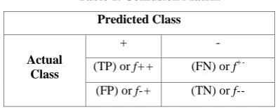
This is a visualization tool which is commonly used to present the accuracy of the classifiers in classification. It is used to show relationships between outcomes and predicted classes
[15]
[image:3.595.322.522.618.695.2]. A confusion matrix is a table at least of size m by m. The table may have additional rows or columns to provide totals or recognition rates per class. True Positives refer to the positive tuples that were correctly labeled by the classifier, while True Negatives are the negative tuples that were correctly labeled by the classifier. False positives are the negative tuples that were incorrectly labeled. False negative are the positive tuples that were incorrectly labeled [16].
Table 1. Confusion Matrix
Predicted Class
Actual Class
+ -
(TP) or f++ (FN) or f +-(FP) or f-+ (TN) or f--
- True positive (TP) or f , which corresponds to the number of positive examples correctly predicted by the classification model.
- False positive (FP) or f which corresponds to the number of negative examples wrongly predicted as positive by the classification model.
- True negative (TN) or f , which corresponds to the number of negative examples correctly predicted by the classification model [16].Formula for measuring Accuracy:
Number of correct predictions Total number of predictions
f f
f f f
Accura y
f c
The error rate can be measured as:
Number of wrong predictions Total number of predictions
f f
f f f
Accura y
f c
4.2
ROC Curve Analysis
ROC is another performance matrix that was used in this study to measure the robustness of the model. It applies to binary classification and requires the designation of a positive class. ROC gains insights into the decision-making ability of a model with an emphasis of how likely is a model to accurately predict the negative or the positive class. ROC measures the impact of changes in the probability threshold. The probability threshold is the decision point used by the model for classification. ROC has been widely used as a performance evaluation tool to measure effectiveness of medical modalities [17].
4.3
Lift Cumulative Positive & Negative
Lift matrix are used to measure the degree to which the classifier prediction of a model are better than randomly generated predictions. Lift is usually applied to binary classification only, and it requires the designation of a positive class. Basically, lift can be understood as a ratio of two percentages: the percentage of correct positive classifications made by the model to the percentage of actual positive classifications in the test data. Lift is normally computed against the quantiles.
4.4 Profit or Loss
A cost matrix encodes the penalty of classifying records from one class as another. Let C(i, j) denotesthe cost of predicting a record from class i as class j. With this notation, C(+,-) is the cost of committing a false negative error, while C(-,+) is the cost of generating a false alarm. A negative entry in the cost matrix represents the reward for making correct classification. Given a collection of N test records, the overall cost of a model M is denoted as:
) , ( ) , ( )
( )
, )
(M TPC FPXC FN C TN C
Ct x x x
5.
RESULTS AND ANALYSIS
5.1
Confusion Matrix Results
Confusion matrix results in table 2 displays the number of correct and incorrect predictions made by the model compared with the actual classifications in the test data. The matrix is n -by-n, where n is the number of classes. The GLM model indicates a 93% of correct predictions with a Correct Prediction Count of 765 patients followed by the SVM‟s count. The SVM model indicates a 84% correct prediction outcome for patients who might be at risk of contracting HIV/ADS related OI with a Correct Prediction count of 690
patients all out of a total case of 820.Table 2. Confusion Matrix Predictions
Model Correct
Predictions%
Correct Prediction Count
In-Correct Prediction Count
Total Case Count
SVM 84.1463 690 130 820
NB 74.7561 613 207 820
GLM 93.297 765 55 820
DT 76.8293 630 190 820
5.2
ROC Curve Performance Results
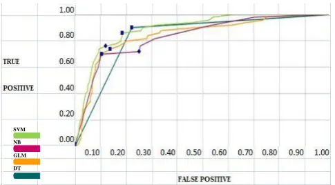
[image:4.595.154.538.94.227.2]The ROC curve performance analysis plots TP (on the y-axis) against FP (on the x-axis) and performance of each classifier is represented as a point on the ROC curve changing the threshold of algorithm. The probability threshold is the decision point used by the model for classification. The results proved that at the 60th quantile, the SVM model had an upper level of accuracy with a maximum overall accuracy of 94.0244%.
Figure 1: ROC Performance results Analysis
Table 3. LIFT performance results
5.3
LIFT Performance Matrix
LIFT performance matrix measures how “fast” a modelfinds the actual positive target values. The Lift viewer compares lift results for the given target value in each model. The Lift viewer displays Cumulative Positive Cases and Cumulative Lift. Table 3 shows a Lift Positive results. In a Lift performance evaluation, the SVM model exhibited the highest cumulative, Gain and Target Density at 3.7356, 82% and 0.2278 respectively.
Model Area
Under Curve
Max Overall Accuracy %
Max Average Accuracy %
SVM 0.839 93.9024 83.8961
NB 0.8472 93.9024 80.1169
GLM 0.8377 93.9024 79.7403
DT 0.8941 94.0244 83.7143
SVM
NB
GLM
[image:4.595.315.558.343.477.2]Table 4. LIFT performance results
Model Lift
Cumulative Gain
Cumulative%
Target Density Cumulative
SVM 3.7356 82 0.2278
NB 3.2398 71 0.197
GLM 3.4622 76 0.2111
DT 3.4167 75 0.2083
5.4
Cost Evaluation Results
[image:5.595.90.244.270.380.2]Cost evaluation results proved that the SVM model has the lowest costing.
Table 5. Cost Evaluation Results
Model
Maximum
Profit
Target Density Cumulative
SVM -1.7317 0.2278
NB -1.7496 0.1975
GLM -2.0976 0.2111
DT -1.8689 0.2083
After performing rigorous testing, comparisons and analysis of the four models, the SVM model performed far much better than the other three models and exhibited a superior performance. The model was therefore applied to the rest of the data and Prediction results were produced.
5.5
SVM Model Deployment
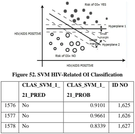
[image:5.595.57.277.538.756.2]SVM had the characteristics of simple classification surface, high generalization performance and high fitting accuracy, etc. SVM is a powerful tool for classification, and it could solve the practical problems, which traditional approaches were incapable of [18].Because of the capability of Oracle miner, the SVM model was applied to the rest of the data and the results available as shown in the figures below:
Figure 52. SVM HIV-Related OI Classification
CLAS_SVM_1_
21_PRED
CLAS_SVM_1_
21_PROB
ID NO
1576 No 0.9101 1,625
1577 No 0.9661 1,626
1578 No 0.8339 1,627
1579 No 0.8839 1,628
1580 No 0.9459 1,629
1581 No 0.8653 1,630
1582 Yes 0.7324 1,631
1583 No 0.8311 1,632
1584 No 0.8631 1,633
1585 Yes 0.8279 1,634
1586 No 0.9111 1,635
1587 No 0.8395 1,636
1588 Yes 0.8685 1,637
1589 Yes 0.5389 1,638
1590 No 0.935 1,639
1591 Yes 0.6714 1,640
1592 No 0.8176 1,641
1593 No 0.9586 1,642
1594 No 0.9851 1,643
1595 No 0.858 1,644
1596 No 0.8435 1,645
1597 No 0.878 1,646
1598 No 0.9157 1,647
1599 No 0.9149 1,648
1600 Yes 0.6355 1,649
Figure 53. SVM HIV-Related OI Classification
Our SVM HIV related OI prediction Model produced results bearing a NO/YES class of whether YES a patient might be at risk of contracting HIV related OI or NO, the Probability rate and the Patients ID number of a patient.
6.
CONCLUSION AND FUTURE WORK
6 positive patients. Although conducting researches on Clinical
data prediction is very vital, there are many challenges that should be taken into consideration. More techniques need to be put in place to ensure that the data is itself healthy from the source level. The HealthCare environment is generally „data rich’ but „information poor‟, compounded with increasing
densities of „data toms‟ which are seldomly visited. More
research work can be done on clinical Big Data Innovations to turn these massive amounts of data into ‘golden nuggets’ of useful information.
7.
ACKNOWLEDGEMENTS
My sincere gratitude goes to Hunan University for having accorded me this opportunity to work on this paper. I would like to acknowledge my Professor Zhiyong Li for his tireless contribution to this paper. I am deeply indebted to the Botswana Government, Ministry of Health in particular for having allowed me to use their data in this research work.
8.
REFERENCES
[1] National Health Act (Act 61 of 2003): Commencement Section 53 of the National Health Act, 2003.
[2] Dubey. A. , Pant. B. , Adlakha. N. “Bioinformatics and Biomedical Technology (ICBBT)”, International Conference on 16-18 April 2010.
[3] Muhammad Usman, “A Methodology for Integrating and Exploiting Data Mining Techniques in the Design of Data Warehouses”, Advanced Information Management and Service (IMS) International Conference, Nov 6th 2010.
[4] Data Mining: Know It All By Soumen Chakrabarti, Earl Cox, Eibe Frank, Ralf Hartmut Güting, Jiawei Han, Xia Jiang, Micheline Kamber, Sam S. Lightsome, Thomas P. Nadeau, Richard E. Neapolitan, Dorian Pyle,Mamdouh Refaat, Markus Schneider, Toby J. Teorey, Ian H. Witten, 2009.
[5] Lilian Sing‟oei1 and Jiayang Wang, School of Information Science and Engineering, Central South University Changsha, 410083, China. “Data Mining Framework for Direct Marketing: A Case Study of Bank Marketing”, IJCSI International Journal of Computer Science Issues, Vol. 10, Issue 2, No 2, March 2013 [6] Irny, S.I. and Rose, A.A. “Designing a Strategic
Information Systems Planning Methodology for Malaysian Institutes of Higher Learning (isp- ipta), Issues in Information System, Volume VI, No. 1, 2005.
[7] Data Mining Know It All by AMSTERDAM • BOSTON • HEIDELBERG • LONDON NEW YORK • OXFORD • PARIS • SAN DIEGO SAN FRANCISCO • SINGAPORE • SYDNEY • TOKYO Morgan Kaufmann is an imprint of Elsevier et al. 2009.
[8] Predictive Analytics: The Hurwitz Victory Index Report Excerpt by Fern Halper, Ph.D Hurwitz & Associates 2011.
[9] Granular Support Vector Machines for Medical Binary Classification Problems by Yuchun Tang, Bo Jin, Yi Sun, and Yan-Qing Zhang, Computational Intelligence in Bioinformatics and Computational Biology , CIBCB 2004.
[10]IBM SPSS Modeler 14.2 Modeling Nodes 1994, 2011. [11]Drug Treatment of HIV-Related Opportunistic Infections
by Dr Michael E. Klepser, Teresa B. Klepser. Springer, January 1997, Volume 53, Issue 1.
[12]Tan P.N, Steinbach M. & Kumar V. Introduction to Data Mining, Pearson Education Inc, 2006 pp.216.
[13]I. Rish, An empirical study of the naive Bayes classifier, T.J. Watson Research Center.
[14]Oracle® Data Mining Concepts 11g Release 2 (11.2) E16808-06 July 2011.
[15]Experimental Comparison of Classifiers for Breast Cancer Diagnosis Gouda I. Salama, M. B. Abdelhalim, and Magdy Abd-elghany Zeid. College of Computing and Information Technology Arab Academy for Science Technology & Maritime Transport Cairo, Egypt. [16]Data Mining Concepts and Techniques by Jiawei and
Micheline Kambler, 2nd Edition p. 360-361, 2006. [17]Granular Support Vector Machines for Medical Binary
Classification Problems by Yuchun Tang, Bo Jin, Yi Sun, and Yan-Qing Zhang, Computational Intelligence in Bioinformatics and Computational Biology , CIBCB 2004.