http://dx.doi.org/10.4236/ojapps.2015.510060
Quantum-Inspired Neural Network with
Quantum Weights and Real Weights
Fuhua Shang
School of Computer and Information Technology, Northeast Petroleum University, Daqing, China Email: [email protected]
Received 28 August 2015; accepted 25 October 2015; published 28 October 2015
Copyright © 2015 by author and Scientific Research Publishing Inc.
This work is licensed under the Creative Commons Attribution International License (CC BY). http://creativecommons.org/licenses/by/4.0/
Abstract
To enhance the approximation ability of neural networks, by introducing quantum rotation gates to the traditional BP networks, a novel quantum-inspired neural network model is proposed in this paper. In our model, the hidden layer consists of quantum neurons. Each quantum neuron carries a group of quantum rotation gates which are used to update the quantum weights. Both input and output layer are composed of the traditional neurons. By employing the back propagation algo-rithm, the training algorithms are designed. Simulation-based experiments using two application examples of pattern recognition and function approximation, respectively, illustrate the availabil-ity of the proposed model.
Keywords
Quantum Computing, Quantum Rotation Gate, Quantum-Inspired Neuron, Quantum-Inspired Neural Network
1. Introduction
still a controversial theory, which has not been experimentally proved. However, the exploration of quantum in-formation devices is a promising research topic, because of the enhanced capacity and speed from the quantum mechanism. With characteristics such as smaller size of quantum devices, larger capacity of quantum networks and faster information processing speed, a quantum neural network can mimic some distinguishing properties of the brain better than the classical neural networks, even if the real human brain does not even have any quantum element. In a word, the quantum neural networks have important research significance in both theory and engi-neering.
Since Kak firstly proposed the concept of quantum neural computation [6] in 1995, the quantum neural net-works had attracted great attention during the past decade, and a large number of novel techniques had been stu-died for the quantum computation and neural networks. For example, Ref. [7] proposed the model of quantum neural networks with multi-level hidden neurons based on the superposition of quantum states in the quantum theory. Ref. [8] proposed a neural network model with quantum gated nodes and a smart algorithm for it, which showed superior performance in comparison with a standard error back propagation network. Ref. [9] proposed a weightless model based on quantum circuit. It is not only quantum-inspired but is actually a quantum NN. This model is based on Grover’s search algorithm, and it can perform both quantum learning and simulate the clas-sical models. Ref. [10] proposes the neural networks with the quantum gated nodes, and indicates that such quantum networks may contain more advantageous features from the biological systems than the regular elec-tronic devices. Ref. [11] have proposed a quantum BP neural networks model with learning algorithm based on the single-qubit rotation gates and two-qubit controlled-NOT gates.
In this paper, we study a new hybrid quantum-inspired neural networks model with quantum weights and real weights. Our scheme is a three-layer model with a hidden layer, which employs the gradient descent principle for learning. The input/output relationship of this model is derived based on the physical meaning of the quan-tum gates. The convergence rate, number of iterations, and approximation error of the quanquan-tum neural networks are examined with different restriction error and restriction iterations. Three application examples demonstrate that this quantum-inspired neural network is superior to the classical BP networks.
2. Quantum-Inspired Neural Network Model
2.1. Qubits and Quantum Rotation GateIn the quantum computers, the “qubit” has been introduced as the counterpart of the “bit” in the conventional computers to describe the states of the circuit of quantum computation. The two quantum physical states labeled as 0 and 1 express 1 bit information, in which 0 corresponds to the bit 0 of classical computers, while 1 bit 1. Notation of “ ” is called the Dirac notation, which is the standard notation for the states in the quantum mechanics. The difference between bits and qubits is that a qubit can be in a state other than 0 and
1 . It is also possible to form the linear combinations of the states, namely superpositions
0 1
φ =α +β (1)
where α and β are complex numbers, called probability amplitudes. That is, the qubit state φ collapses
into either 0 state with probability α2, or 1 state with probability β 2, and we have
2 2
1
i i
α + β = . (2)
Hence, the qubit can be described by the probability amplitudes as
[
α β,]
T.Suppose we have n qubits, and correspondingly, a n qubits system has 2n computational basis states. Similar to the case of a single qubit, the n qubits system may form the superpositions of 2n basis states:
( )0,1n x
x a x
φ =
∑
∈ (3)where ax is called probability amplitude of the basis states x , and “
{ }
0,1 ” means “the set of strings of length two with each letter being either zero or one”. The condition that these probabilities can sum to one is expressed by the normalization condition( ) 2 0,1n x 1
x∈ a =
In the quantum computation, the logic function can be realized by applying a series of unitary transform to the qubit states, which the effect of the unitary transform is equal to that of the logic gate. Therefore, the quantum services with the logic transformations in a certain interval are called the quantum gates, which are the basis of performing the quantum computation.
The definition of a single qubit rotation gate is given
( )
cos sinsin cos
R θ θ θ
θ θ
−
=
. (5)
Let the quantum state 0 0 cos
sin
θ φ
θ
=
, and φ can be transformed by R
( )
θ as follows:( )
(
(
0)
)
0 cos
sin
R θ φ θ θ
θ θ
+
= +
(6)
It is obvious that R
( )
θ shifts the phase of φ .2.2. Quantum-Inspired Neuron Model
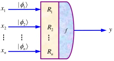
A neuron can be described as a four elements array: (input, weight, transform function, output), where input and output is the outer attribute of the neuron, and weight and transform function are the inner attribute of the neuron. Therefore, the different neuron models can be constructed by modifying types of weight and transform function. According this viewpoint, for the quantum-inspired neuron proposed in this paper, the weights are represented by qubits, and the transform function is represented by inner-product operator. The difference from the tradi-tional neuron is that the quantum-inspired neuron carries a group of single-bit quantum gates that modify the phase of quantum weights. The quantum-inspired neuron model is shown in Figure 1.
In quantum-inspired neuron model, the weights are represented by qubits φi =αi 0 +βi 1 =
[
α βi, i]
T. Let(
)
T1, 2, , n
X = x x x is the input real vector, y is an output real number, φi =
[
α βi i]
Tis the quantum weight, the input/output relation of quantum-inspired neuron can be described as follows:(
)
1n i i i i
y= f XRφ = •C
∑
= x R φ (7)where • is an inner product operator, f X
( )
= •C X , C=[ ]
1 , 1T, the Ri is a quantum rotation gate tomodify the phase of the φi .
2.3. Quantum-Inspired Neural Network Model
[image:3.595.215.413.601.707.2]Quantum-inspired Neural Network (QINN) is defined as the model that all the input, output, and linked weights for each layer may be qubits. The QINN structure is the same as the general ANN which includes input layer, hidden layer, and output layer. Obvious, the network including neuron in Figure 1is QINN. The QINN only in-cluding quantum neurons is defined as the normalization QINN, and the QINN inin-cluding quantum neurons and general neurons is defined as the hybrid QINN. Since QINN transform function adopts linear operator, the non-
Figure 1. Quantum-inspired neuron model.
1
R
2
R
n
R
1
x
2
x
n
x
┇ ┇ ┇
〉
1
|
φ
y
〉
2
|
φ
〉
n
φ
|
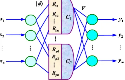
linear mapping capability falls under restriction. Therefore, this paper considers the hybrid QINN (HQINN) in-cluding a hidden layer of quantum neuron, which holds the advantage of the quantum computing and the nonli-near mapping capability of the general ANN. HQINN model is presented in Figure 2.
The model includes three layers, the input layer and output layer contains n and m general neurons, respec-tively, and the hidden layer contains p quantum-inspired neurons. The input/output relation can be described as follows:
(
11)
nj j i i ij ij
p
k j jk j
h C x R
y g v h
φ = = = • =
∑
∑
(8)where i=1, 2,,n; j=1, 2,,p; k=1, 2,,m, vjk is the linked weight between the jth neuron in hidden layer and the kth neuron in output layer, g is the Sigmoid function or Gauss function.
2.4. Learning Algorithm
For the HQINN in Figure 2, when transform function in output layer is continuous and differentiable, the learn-ing algorithm may adopt BP algorithm. The output error function is defined as follows:
(
)
21 1 ˆ 2 m k k k
E=
∑
= y −y (9)where ˆyk represents the desired output.
According to BP algorithm, the modifying formula for output layer weight is described as follows:
(
1)
( )
( )
1(
ˆ( )
)
( ) ( )
jk jk jk k k j
jk
E
v t v t v t y y t g t h t
v
η ∂ η ′
+ = + = + −
∂ (10)
where, j=1, 2,,p, k=1, 2,,m, η represents the learning ratio, and t represents the iteration steps. The weights between the input layer and quantum hidden layer are modified by quantum rotation gates de-scribed as follows:
( )
( )
( )
( )
cos sin sin cos ij ij ij ij ij R θ θ θ θ ∆ − ∆ = ∆ ∆ (11)where i=1, 2,,n, j=1, 2,,p. According BP algorithm, the ∆θij can be gained from the following for-mula.
( )
(
( )
)
( ) ( ) ( )
(
(
( )
)
(
( )
)
)
1 1
ˆ cos sin
m m
j k
ij k k jk j i ij ij
k k
ij k j ij
h y
E E
t y y t g t v t h t x t t
y h
θ ϕ ϕ
θ = θ =
∂ ∂
∂ ∂ ′
∆ = = − = − − −
∂
∑
∂ ∂ ∂∑
(12) [image:4.595.208.422.566.703.2]where ϕij
( )
t is the phase of the φij . For ϕij( )
t , the modifying formula is described as follows.(
1)
( )
( )
ij t ij t ij t
ϕ + =ϕ + ∆θ (13)
Let the vector φij = α βij, ijT, the modifying formula of φij is described as follows:
(
)
(
)
( )
( )
( )
( )
( )
( )
cos sin
1
1 sin cos
ij ij
ij ij
ij ij ij ij
t t
t t
θ θ
α α
β θ θ β
∆ − ∆
+
=
+ ∆ ∆
(14)
where t represents the iteration steps.
Synthesizing above depiction, the HQINN learning algorithm can be described as follows:
Step 1: Initialize network parameters. Include: The number of nodes in each layer, the learning ratio, the re-striction error ε, the restriction steps Max. Set the current steps t=0.
Step 2: Initialize network weights. Hidden layer: ϕij
( )
t =2π×rnd,( )
(
)
( )
(
)
cos
sin ij ij
ij
t
t
ϕ φ
ϕ
=
, and output layer:
0.5 jk
v =rnd− , where rnd is a random number in (0,1), i=1, 2,,n, j=1, 2,,p, k=1, 2,,m.
Step 3: Compute network outputs according to Equation (8), modifying the weights of each layer according to Equation (10) and Equation (14), respectively.
Step 4: Compute network output error according to Equation (9), if E<ε or t>Max then go to Step 5, else t= +t 1, go back to Step 3.
Step 5: Save the weights, and stop 3.
3. Simulations
To testify the validity of HQINN, two kinds of experiments are designed and the HQINN is compared with the classical BP network in this section. In two experiments, the HQINN adopts the same structure and parameters as the BP network.
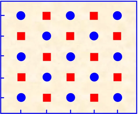
3.1. Twenty-Five Sample Patterns Classification
For twenty-five sample points in Figure 3, determine the pattern of each point by HQINN. This is a typical two-pattern classification problem, which is regard as the generalization of XOR problem.
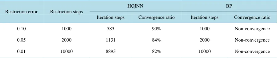
The network construct is set to 2-10-1, and the learning ratio is set to 0.8. The HQINN and the BP network are learned 50 times, restively, and then compute the average of iteration steps. Training results are shown in
[image:5.595.195.433.506.703.2]Table 1. When the restriction error takes 0.05, the convergence curves are shown in Figure 4.
Figure 4. The convergence curve comparison.
Table 1. The training results comparison between HQINN and BP network for 25 sample patterns classification.
Restriction error Restriction steps
HQINN BP
Iteration steps Convergence ratio Iteration steps Convergence ratio
0.10 1000 583 90% 1000 Non-convergence
0.05 2000 1131 84% 2000 Non-convergence
0.01 10000 8893 82% 10000 Non-convergence
3.2. Double Spiral Curves Classification
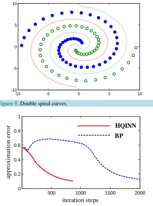
For two spiral curve in Figure 5, fetch 30 points from each curve, respectively, compose the sample set con-taining 50 sample points, and classify these points in sample set by HQINN.
The network construct is 2-20-1, and the learning ratio is 0.7. The HQINN and the BP network are training 30 times, restively, and then compute the average of iteration steps. Training results are shown inTable 2. When the restriction error takes 0.10, the convergence curves are shown in Figure 6.
3.3. Function Approximation
In this simulation, such function is selected as follow:
(
)
21.5
1 2 3
1.0 1
y= + x + x +x− (20)
where x1, x2, and x3 are integers in the set {1, 2, 3, 4, 5}.
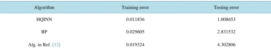
To approximate the nonlinear function, we sample 40 groups of discrete data, half of which is used to train networks and the other half to test its performance. Set the maximum of iteration steps 5000. By changing the number of hidden neurons and the learning coefficient, we present an experimental evaluation of HQINN’s and compare their performance with that of the other algorithms. This example is simulated 30 times for each group of parameters by the HQINN, the BP, and the algorithm in Ref. [12], respectively. When the number of hidden neurons is 6 and 8, the training result are presented inTable 3 andTable 4.
Firstly, we investigate how to change for the average convergence rate when the learning coefficient changes. The networks structure is 3-5-1, the restriction error is 0.1, and the restriction iteration steps are 5000. The learning coefficient set is {0.1, 0.2, …, 1.0}. This example is simulated 30 times for each learning coefficient by the HQINN and the BP respectively. When the learning coefficient changes the average convergence ratio of HQINN always is 100% and is insensitive to the learning coefficient. However, the average convergence ratio of BP changes in a large range when the learning coefficient changes. The maximum of average convergence ratio of BP reaches to 80%, and the minimum is only 10%. The comparison result is shown in Figure 7.
The comparison result shows that the HQINN is evidently superior to the BP in both the average convergence ratio and the robustness.
500 1000 1500 2000
0 0.2 0.4 0.6 0.8 1
iteration steps
a
ppr
oxi
m
a
ti
on e
rr
or HQINN
[image:6.595.89.539.266.360.2]Figure 5. Double spiral curves.
Figure 6.The convergence curve comparison.
[image:7.595.89.540.647.720.2]Figure 7. The relationship between the average convergence rate and the learning coefficient.
Table 2.The training results comparison between HQINN and BP network for double spiral curves classification.
Restriction error
Restriction steps
HQINN BP
Iteration steps Convergence ratio Iteration steps Convergence ratio for convergence Necessary steps
0.10 2000 871 82% 2000 Non-convergence 3961
0.05 10000 6893 92% 8631 76% —
-10 -5 0 5 10
-10 -5 0 5 10
500 1000 1500 2000
0 0.2 0.4 0.6 0.8 1
iteration steps
a
ppr
oxi
m
a
ti
on e
rr
or HQINN
BP
0 0.2 0.4 0.6 0.8 1
0 20 40 60 80 100
Learning coefficient
A
v
er
age c
onv
er
genc
e r
at
io (
%
)
Secondly, we investigate how to change for the average iteration steps when the learning coefficient changes. The networks structure is 3-5-1, and the restriction error is 0.1. The learning coefficient set is still {0.1, 0.2, …, 1.0}. This example is simulated 30 times for each learning coefficient by the HQINN and the BP, respectively. When the learning coefficient changes, for the average iteration steps of HQINN, the maximum is 958 steps, the min-imum is 496 steps, and the average is 693 steps. However, for the average iteration steps of BP, the maxmin-imum is 4619 steps, the minimum is 1532 steps, and the average is 2489 steps. Hence, the performance of HQINN is evidently superior to BP in both the average iteration steps and its fluctuation range when the learning coeffi-cient changes. The comparison result is shown inFigure 8.
The comparison results show that the HQINN is evidently superior to the BP in both the average iteration steps and the robustness.
4. Conclusion
The HQINN is the amalgamation of quantum computing and nerve computing, which holds the advantage such as parallelism and high efficiency of quantum computation besides continuity, approximation capability, and generalization capability that the classical ANN holds. In HQINN, the weights are represented by qubits, and the phase of each qubit is modified by the quantum rotation gate. Since both probability amplitudes participate in optimizing computation, the computation capability is evidently superior to the classical BP network. Experi-mental results show that the HQINN model proposed in this paper is effective.
Figure 8. The relationship between the average iteration steps and the learning coefficient.
Table3. The simulation result for the nonlinear function approximation (the number of hidden neurons is 6).
Algorithm Training error Testing error
HQINN 0.035236 0.635218
BP 0.083605 3.268351
Alg. in Ref. [12] 0.019852 1.775031
Table4.The simulation result for the nonlinear function approximation (the number of hidden neurons is 8).
Algorithm Training error Testing error
HQINN 0.011836 1.008653
BP 0.029605 2.831532
Alg. in Ref. [12] 0.019324 4.302806
A
v
er
ag
e ite
ra
tio
n
s
te
p
s
Learning coefficient 1000
2000 3000 4000 5000
0.0 0.2 0.4 0.6 0.8 1.0
HQINN
[image:8.595.90.537.636.720.2]Acknowledgements
This work was supported by the National Natural Science Foundation of China (Grant No. 61170132), the Scien-tific research and technology development project of CNPC (2013E-3809), and the Major National Science and Technology Program (2011ZX05020-007).
References
[1] Benioff, P. (1982) Quantum Mechanical Hamiltonian Models of Turing Machines. Journal of Statistical Physics, 3, 515-546. http://dx.doi.org/10.1007/BF01342185
[2] Shor, P.W. (1994) Algorithms for Quantum Computation: Discrete Logarithms and Factoring. Proceedings of the 35th Annual Symposium on Foundations of Computer Science, Santa Fe, 20-22 November 1994, 124-134.
http://dx.doi.org/10.1109/SFCS.1994.365700
[3] Grover, L.K. (1996) A Fast Quantum Mechanical Algorithm for Database Search, Proceedings of the 28th Annual ACM Symposium on the Theory of Computing, Pennsylvania, May 1996, 212-219.
http://dx.doi.org/10.1145/237814.237866
[4] Penrose, R. (1994) Shadows of the Mind: A Search for the Missing Science of Consciousness. Oxford University Press, London, 196-201.
[5] Penrose, R. (1989) The Emperor’s New Mind: Concerning Computers, Minds, and the Laws of Physics. Oxford Uni-versity Press, London, 89-93.
[6] Kak, S. (1995) On Quantum Neural Computing. Information Sciences, 83, 143-160.
http://dx.doi.org/10.1016/0020-0255(94)00095-S
[7] Gopathy, P. and Nicolaos B.K. (1997) Quantum Neural Networks (QNN’s): Inherently Fuzzy Feed Forward Neural Networks. IEEE Transactions on Neural Networks, 8, 679-693. http://dx.doi.org/10.1109/72.572106
[8] Li, P.C., Song, K.P. and Yang, E.L. (2010) Model and Algorithm of Neural Network with Quantum Gated Nodes. Neural Network World, 11, 189-206.
[9] Adenilton, J., Wilson, R. and Teresa, B. (2012) Classical and Superposed Learning for Quantum Weightless Neural Network, Neurocomputing, 75, 52-60. http://dx.doi.org/10.1016/j.neucom.2011.03.055
[10] Shafee, F. (2007) Neural Networks with Quantum Gated Nodes. Engineering Applications of Artificial Intelligence, 20, 429-437. http://dx.doi.org/10.1016/j.engappai.2006.09.004
[11] Li, P.C. and Li, S.Y. (2008) Learning Algorithm and Application of Quantum BP Neural Networks Based on Universal Quantum gates. Journal of Systems Engineering and Electronics, 19, 167-174.
http://dx.doi.org/10.1016/S1004-4132(08)60063-8
![Crystal structure of ethyl 5 (3 fluorophenyl) 2 [(4 fluorophenyl)methylidene] 7 methyl 3 oxo 2H,3H,5H [1,3]thiazolo[3,2 a]pyrimidine 6 carboxylate](data:image/gif;base64,R0lGODlhAQABAIAAAP///wAAACH5BAEAAAAALAAAAAABAAEAAAICRAEAOw==)