Simulation and Comparison of Various Lossless Data Compression Techniques based on Compression Ratio and Processing Delay

Volume 81 – No 14, November 2013

Simulation and Comparison of Various Lossless Data

Compression Techniques based on Compression Ratio

and Processing Delay

Dhananjay Patel

Don Bosco Institute Of Technology, Mumbai

Vinayak Bhogan

Don Bosco Institute Of Technology,Mumbai

Alan Janson

Don Bosco Institute Of Technology, Mumbai

ABSTRACT

With increasing need to store data in lesser memory several lossless compression techniques are developed. This paper intends to provide the performance analysis of lossless compression techniques over various parameters like compression ratio, delay in processing, size of image etc. It provides the relevant data about variations in them as well as to describe the possible causes for it. It describes the basic lossless techniques as Huffman encoding, run length encoding, arithmetic encoding and Lempel-ziv-welch encoding briefly with their effectiveness under varying parameters. Considering the simulation results of grayscale image compression achieved in MATLAB software, it also focused to propose the possible reasons behind differences in comparison.

General Terms

Image compression, Lossless compression techniques, Huffman, Arithmetic, Lempel-ziv-welch (LZW), Run length Coding (RLE).

Keywords

Compression Ratio, Probability of Zero and Processing Delay.

1.

INTRODUCTION

The storage of data using minimum memory is always a problem. A digital image obtained after the process of sampling and quantizing of a continuous tone picture requires an enormous storage space. For Example a 1024x1024 pixels image requires normally 1Megabyte of space. To overcome this storage issue and to make proper management of space various image compression techniques were developed. Image compression is a process of reducing the amount of data required to represent a sampled digital image thereby reducing the cost for storage and transmission without degrading the quality of the image to an unacceptable level [1] [9].

The important applications of Image compression such as including image database, image communications and time reduction required for images to be sent over the Internet or downloaded from Web pages.

The important parameter of the image compression techniques is compression ratio. It is defined as the ratio of the original image size to the compressed image size. For example an image of 100x100 pixels will require normally 10KB of size but after compression the size becomes 5KB. Hence the compression ratio is 2. A good compression technique should have compression ratio greater than 1. To achieve this many image compression were developed.

Image compression Techniques are broadly divided into 2 types such as “lossless” and “lossy”. In lossless compression,

the original data should be same after the compression has occurred. Text File are stored using lossless compression techniques since because loss of a single character can change the meaning and will lead to improper information. The group storage of sources for images, audio data and video data generally needs to be lossless as well.

Lossless compression techniques cannot give much compression as lossy compression techniques can give. In lossy compression, much information can be simply discarded away from image, audio data and video data and when they are uncompressed the data will still be of acceptable quality. Lossy compression techniques can give much greater compression ratio then the lossless compression available for given image data, audio data and video data [1].

Some of the lossless compression techniques are

1. Huffman Coding

2. Arithmetic coding

3. RLE

4. LZW

2.

COMPRESSION TECHNIQUES

2.1

Huffman coding

It is a fixed length coding technique which is coded for the symbols based on their statistical occurrence frequencies that is the probability. Symbols are generated on the basis of pixels in an image. On the basis of its frequently occurrence, bits are assigned to it. Less bits are assigned to symbols that occurs more frequently while larger number of bits are assigned to symbols that occur less. In Huffman codes the generated binary code of any symbol is not the prefix of the code of any other symbol [4] [2].

Implementing Huffman coding on MATLAB v7.12 (R2011a), following steps are executed [10]:

1. Read a greyscale image & convert the array into single row vector.

2. Form a Huffman encoding tree using probability of symbols in gray scale image read.

3. Encode each symbol independently using the encoding tree.

Volume 81 – No 14, November 2013

32

2.2

Run length coding

This is one of the simplest compression techniques used for compression of repeated or sequential data. In this technique, it scans for a repeated symbol that is pixels in an image and replaces it by a shorter symbol called “run”. Hence it is known as run length encoding. This redundancy is used for compression. For a gray scale image, the run length code is represented by {Si, Ci} where Si is the symbol or intensity of pixels and Ci is the count or the number of repeated symbol Si occurred. This compression technique is useful for monochrome images or images having of same background pixels. Generally, all pixels are first converted into binary values & then individual counts of consecutive zeroes & ones are stored, known as run length encoding [2].

To implement the run length encoding in MATLAB following steps are executed:

1. Read the gray scale image and rearrange data of image as single row vector.

2. Convert all intensities values to binary state & obtain a binary stream representation of image.

3. Count consecutive 1’s & 0’s appeared in a sequence and stored as run length encoded sequence.

4. Get the compression ratios using original size of image and size of run length encoded sequence.

2.3

Arithmetic encoding

Arithmetic coding is also a variable length coding technique. In this compression technique, it converts the entire symbols generated from the pixels into a single floating point number also termed as binary fraction. In arithmetic coding technique, a tag is generated for the sequence which is to be encoded. This tag signifies the given binary fraction and becomes the unique binary code for the sequence. This unique binary code generated for a given sequence of length L is not depended on the entire sequence of length L [2] [3] [9].

The results are generated using following algorithm steps that are followed during practical implementation of arithmetic encoding in MATLAB [11].

1. Read the image & store all intensity values as a single

row vector.

2. Convert the matrix into binary form and arrange all bits

in binary stream representing the same image.

3. Encode the entire stream using arithmetic encoding tree

algorithm

4. Get the compression ratios using size of original image and the size of encoded image.

2.4

Lempel-Ziv-Welch (LZW) coding

LZW known as Lempel-Ziv-Welch is an image compression technique is based on “Dictionary”. Dictionary based coding scheme are of two types, Static and Adaptive. In Static Dictionary based coding, dictionary size is fixed during encoding and decoding processes and in Adaptive Dictionary based coding; dictionary size is updated and reset when it is completely filled. Since we use images as data, static coding suits fine for the compression job with minimum delay [2] [5] [6].

In order to obtain results, following steps are executed in MATLAB [5][6]:

1. Read an image & arrange all intensity value in single row vector.

2. Convert all the values in binary for & achieve a single row binary representation of same image.

3. Initialize dictionary with basic symbols viz 1 & 0.

4. Start encoding & decoding based on search & find method. Add any new word found in dictionary & encode the sequence.

5. If dictionary is completely filled, continue using same dictionary.

6. Get the compression ratios using size of original image & size of encoded sequence.

3.

EVALUATION AND COMPARISON

3.1

Results with real images

Table 1: Compressionratio with real images

Table 2:Bits per pixel with real images

As seen in the table 1 and table 2, the relative compression ratios and bits per pixel are displayed with respect to each technique used for compression. Among all, the run length shows minimum compression ratio and also bits per pixel because run length algorithm simply works to reduce inter-pixel redundancy which exists only when extreme shades are significant. Since with most of the real world images lack such dominance of shades, run length is totally obsolete technique for lossless data compression. Considering the available data about compression ratio, Huffman encoding scheme is found to be optimum since it solely works on reducing redundancy in input data. However, though it seems that Arithmetic also generates closest results as Huffman encoding, it also considers inter-pixel redundancy which reduces the compression factor in case of real images. Lempel-Ziv-Welch encoding totally works on dictionary size

Image size Huffman Run Length Arithmatic LZW dictionary size = 512

Face 32 x 32 1.1034 0.29889 1.0049 0.9258

Keyboard 48 x 48 1.1791 0.2321 1.0034 0.9446

Airpacific 64 x 64 3.0704 1.1145 2.2667 2.7788

Vegitables 128 x 128 1.0435 0.2283 1.0015 0.9686

Einstein 153 x 153 1.1244 0.2348 1.0013 0.9683

Horses 160 x 160 1.0479 0.2326 1 0.973

Moon 240 x 240 1.389 0.3481 1.1179 1.1635

Image

Size

Huffman Run Length Arithmatic

LZW

dictionary size = 512

Face

32 x 32 7.2503

26.765

7.9609

8.6411

Keyboard 48 x 48 6.7848

34.4679

7.9728

8.4691

Airpacific

64 x 64 2.6055

7.1781

3.5293

2.8789

Vegitables 128 x 128 7.6665

35.0416

7.988

8.2593

Einstein

153 x 153 7.1149

34.0715

7.9896

8.2619

Horses

160 x 160 7.6343

34.393

8

8.2219

Volume 81 – No 14, November 2013 as a key factor to achieve greater compression ratios. Thus

with lower dictionary sizes the compression results are still lower as compared to other compression techniques.

3.2

Compression ratio against probability

of zero

This paper discusses all the essential differentiation between Huffman, run length, arithmetic& Lempel-Ziv-Welch compression techniques using images as data. The comparisons are dealing with some important parameters viz. compression ratio & delay in processing. In order to develop comparative data for each one, simulations of compression techniques were performed on MATLAB software using random images.

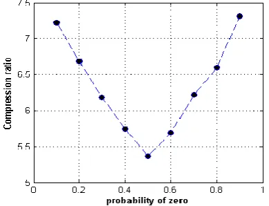
The variations of compression ratio & probability of zero are achieved by generating random images of same size 50x50 pixels while changing probabilities for symbol zero in each by 0.1.

Fig 1: Compression ratio against probability for Huffman coding

Fig 2: Compression ratio against probability for Run length coding

Fig 3: Compression ratio against probability for Arithmetic coding

Fig 4: Compression ratio against probability for LZW coding

The Fig 1, 2, 3& 4 shows variation of compression ratio with probability of zero (i.e zero symbol) in the image to be compressed. As the probability zero approaches to zero the compression ratio decreases. Irrespective of technique used for compression the results are similar showing minimal compression ratio at probability of zero as 0.5. This indeed closely can be related to the standard entropy of any binary data with respect to probability of occurrences of symbols. When probability of zero & one in given data is equal (each as 0.5) the content of information is maximum. As we tend to move towards extreme probabilities the redundancy in information becomes more & more significant. Thus by any lossless technique, the compression results are best when probabilities of symbols lie to either extreme probabilities.

Volume 81 – No 14, November 2013

34

3.3

Delay performance

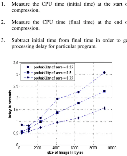
Results are achieved by compressing random images of different sizes but same probabilities. Three distinct data sets are generated with probability of symbol zero as 0.25 0.5 & 0.75.It’s obvious that as size of image increases the time required for compression or processing delay also increases. But delay profile shows changes when there is any change in probability of zero while keeping size variation same.

Steps followed to measure delay are

1. Measure the CPU time (initial time) at the start of compression.

2. Measure the CPU time (final time) at the end of compression.

3. Subtract initial time from final time in order to get processing delay for particular program.

Fig 5: Processing delay variations against size of image for Huffman encoding

In the Fig 5 processing delay reduces as we increase probability of zero in image for Huffman coding. For Huffman compression technique, the compression is basically rearrangement of bits as per the content of information. When the symbol zero has probability less than 0, Huffman coding will assign 1 to it. Now as per the Huffman encoding tree structure in MATLAB, the coding will firstly be done to assignment 0 & then assignment 1.Thus more the no of zeroes, more the assignment 1 in coding table & more is the delay for encoding entire data. Same can be applied in reverse way when probability of zero crosses the equi-probable point

.

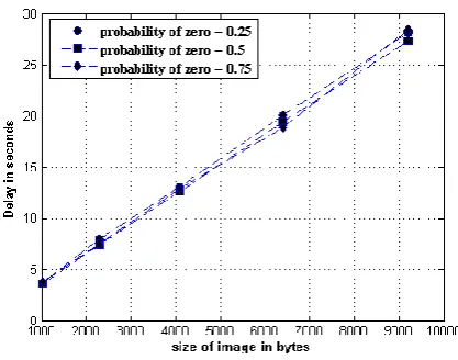
Fig 6: Processing delay variations against size of image for Run length encoding

In the Fig 6showing processing delay profile for run length compression technique, delay in processing is independent on probability of zero. The Principle of run length encoding is simply counting number of same symbols (both 0’s as well as 1’s) in sequence. Thus whatever may be probability of zero, the encoding process has no effect & hence no delay variations are observed with variation in probability of zero for same image size.

Fig 7: Processing delay variations against size of image for Arithmetic encoding

Volume 81 – No 14, November 2013

Fig 8: Processing delay variations against size of image for LZW encoding

Compression technique of LZW is totally based on the formation of dictionary rather than other probability dependent techniques. Thus in Fig 8 it can be easily found that processing delays are almost same for any given image size irrespective of the probability of symbols.

4.

CONCLUSION

From above implementation & simulation we conclude

1) With findings of real images, Huffman is better than other techniques since it follows optimal method to remove redundancy from given data.

2) From evaluation of compression ratio against probability of zero in data, compression ratio achieved would be maximum if one of the symbols has much greater probability in data. In other words, more the entropy lesser the compression achieved for data.

3) From relative comparison of processing delay, for the techniques which focuses on removal of redundancy in data like Huffman & arithmetic, probabilities of symbol affects delay in processing. But those techniques which are dictionary based/inter-pixel redundancy based do not show any significant change in delay with change probability of symbol.

5.

REFERENCES

[1] Mohammed Al-laham1 & Ibrahiem M. M. El Emary2, “Comparative Study BetweenVarious Algorithms of Data Compression Techniques”, Proceedings of the World Congress on Engineering and Computer Science 2007 WCE CS 2007, October 24-26, 2007, San Francisco, USA.

[2] Sonal Dinesh Kumar, “A Study Of Various Image CompressionTechniques”, Proceedings of COIT, RIMT Institute of Engineering and Technology, Pacific, 2000, pp. 799-803.

[3] Amir said, “Introduction to arithmetic coding- theory and practice”,Imaging System Laboratory HP Laboratories Palo Alto HPL-2004-76, April 21,2004.

[4] Huffman D.A., “A method for the construction of minimumredundancycodes”, Proceedings of the Institute of RadioEngineers, 40 (9), pp. 1098–1101, September 1952.

[5] Ziv. J and Lempel A., “A Universal Algorithm for Sequential Data Compression”, IEEE Transactions on Information Theory 23 (3), pp. 337–342, May 1977. [6] Ziv. J and Lempel A., “Compression of Individual

Sequences via Variable-Rate Coding”, IEEE Transactions on InformationTheory 24 (5), pp. 530–536, September 1978.

[7] Subramanya A, “Image CompressionTechnique,” Potentials IEEE, Vol. 20, Issue 1, pp 19-23, Feb-March 2001.

[8] David Jeff Jackson & Sidney Joel Hannah, “Comparative Analysis of image Compression Techniques,” System Theory 1993, Proceedings SSST’93, 25th Southeastern Symposium,pp 513-517, 7 –9March 1993.

[9] Khalid Sayood, “Introduction to Data Compression”, 3nd Edition,San Francisco, CA, Morgan Kaufmann, 2000.

[10]Dr. T. Bhaskara Reddy, Miss. Hema Suresh Yaragunti , Dr. S. Kiran, Mrs. T. Anuradha , “A Novel Approach of Lossless Image Compression using Hashing andHuffman Coding”, International Journal of Engineering Research & Technology (IJERT) ISSN: 2278-0181, Vol. 2 Issue 3, March – 2013.