Design of Digital IIR Filters using Integrated Cat Swarm
Optimization and Differential Evolution
Kamalpreet kaur
Department of Electrical and Instrumentation Engineering,
Sant Longowal Institute of Engineering and Technology,
Longowal-148106, Punjab, India
J. S. Dhillon
Department of Electrical and Instrumentation Engineering,
Sant Longowal Institute of Engineering and Technology,
Longowal-148106, Punjab, India
ABSTRACT
This paper aims to establish a solution methodology for the optimal design of digital infinite impulse response (IIR) filters by integrating the features of cat swarm optimization (CSO) and differential evolution algorithm (DE). DE is a population based stochastic optimization technique which optimizes real valued functions. It requires negligible control parameter tuning but sometimes causes instability problem. CSO is a heuristic optimization algorithm based on the observations and imitation of the natural behavior of cats. CSO algorithm possesses local as well as global search capabilities. Although, CSO possesses better capability to search optimal point but it requires a higher computation time because the local and global searches are carried out independently in each iteration. A hybrid algorithm is proposed using the CSO algorithm and the DE optimization algorithm for the robust and stable design of digital IIR filter. To start with a better solution set, opposition based learning strategy is incorporated. The proposed method explores and exploits the search space locally as well as globally. The design criterion undertakes the minimization of magnitude approximation error and ripple magnitudes of both pass-band and stop-band satisfying the stability requirements. The developed hybrid algorithm is effectively applied for designing the digital low-pass, high-pass, band-pass and band-stop filters. The computational results demonstrate that the proposed algorithm is capable of creating designs that are competitive with reference to other design processes and can efficiently be applied for higher order filter design.
Keywords
Digital IIR filters, cat swarm optimization, differential evolution, multiparameter optimization, opposition based learning.
1.
INTRODUCTION
Digital filters allow a certain band of frequency to pass through them, while attenuating the other frequencies in order to suppress interfering signals and reduce background noise. Generally speaking, there are two types of digital filters, i.e. finite impulse response (FIR) and infinite impulse response (IIR). Compared with an FIR filter design problem, an IIR filter design problem is more challenging. The design task of IIR digital filters is to approximate a given ideal frequency response by a stable IIR digital filter under some design criterion. If both magnitude and phase/group delay responses are considered, an IIR digital filter design problem is essentially a non-convex optimization problem due to the presence of the denominator of the transfer function [28]. Digital IIR filters often provide a much better performance and less computational cost than their equivalent FIR filters and have become the target of growing
interest. The motivation for using the IIR filters is that they usually have much sharper roll-offs in their frequency responses than the FIR filters of equal complexity.
There are mainly two approaches to design digital IIR filter, namely: (i) transformation approach and (ii) optimization approach. The transformation approach involves the transformation of an analog filter to a digital filter for a given set of prescribed specifications [31]. But the performance of digital IIR filters designed by using the transformation approach is not good as they require too much pre-knowledge and return a single solution in most of the cases. In the optimization approach, various optimization methods have been proposed to obtain optimal filter performances, where the magnitude approximation error, mean-square-error, and ripple magnitudes of both pass band and stop band are usually used as criteria to measure the performance of the designed digital IIR filters. IIR filters are generally multimodal with respect to the filter coefficients and the conventional gradient-based algorithm easily stuck at local minima [8]. In order to overcome the shortcomings of conventional methods and to achieve a global optimal solution, in recent years many nature inspired optimization algorithms have been implemented for the digital IIR filter design problem.
Genetic algorithm (GA) has been successfully applied by Tang et.al. [7] and Li et.al [5] for the design of digital IIR filter. A hybrid Taguchi genetic algorithm (HTGA) has been proposed by Tsai et.al. [16] for the design of optimal digital IIR filters. The HTGA approach is a method which is obtained by combining the traditional genetic algorithm, which has a powerful global exploration capability, with the Taguchi method, which can exploit the optimum offspring. Afterwards, Tsai et.al. [17] integrated the immune algorithm with the Taguchi method and proposed a hybrid algorithm named Taguchi-immune algorithm (TIA) for optimal digital IIR filter design. Kaur et.al. [39] have used the real coded genetic algorithm (RCGA) for digital IIR filter design. Poor precision is followed by a binary coded parameter as sometimes it skips the best solution in the coding process [39].
the transition band and finds the lowest filter order simultaneously but may require too many function evaluations. Ant colony optimization algorithm has been proposed by Karaboga et.al. [12] for the design of digital IIR filter. This method possesses global optimization ability and is a modified version of tourism ant colony optimization algorithm which has been particularly introduced for continuous optimization. In continuation; they presented a method based on immune algorithm for the digital IIR filter design and compared its performance with the ant colony optimization algorithm, tabu search and genetic algorithm [13]. The immune algorithm method has the ability of finding global optimal solution in a nonlinear search space but suffer from the problems of search stagnation and premature convergence [13].
Particle swarm optimization is population based optimization technique developed by Eberhart and Kennedy [3] inspired by natural behavior of bird flocking and fish schooling. It is a computationally fast algorithm and has robust search ability. Del et. al. [21] presented a detailed review of the Particle swarm optimization. The conventional Particle swarm optimization algorithm encountered a problem in which it loses global search ability. To overcome this problem Silva et. al. [9] proposed the predator-prey optimization (PPO) algorithm and tested it to some benchmark problems. They concluded that PPO method performed effectively better than the PSO on many of these problems. Still, PPO has not been applied to constrained optimization problems which are getting quite attention in these days for digital IIR filter design.
Nowadays, for solving complex optimization problems, population based algorithms like evolutionary algorithms (EAs), Particle swarm optimization (PSO), PPO and DE are being used. DE is a very simple, powerful, stochastic, population-based, easy to use optimization algorithm, which has been developed to optimize the real valued parameter and functions. Storm and Price [4] introduced the differential evolution algorithm (DE) and successfully applied it for the optimization of some well-known nonlinear, non-differentiable, and non-convex functions. Das and Suganthan [29] provided an extensive overview of the various engineering applications that have benefited from the powerful nature of DE algorithm. Differential evolution algorithm has a number of significant advantages. It has the ability to find the true global minimum regardless of the initial parameter values. It possesses parallel processing, requires only few control parameters and results in fast convergence. DE is capable of providing multiple solutions in a single run and has ability to find the optimal solution for a nonlinear constrained optimization problem with penalty functions. In contrast to these advantages DE has a number of disadvantages too. In DE, there exist many trial vector generation strategies out of which a few may be suitable for solving a particular problem. Moreover, three crucial control parameters involved in differential evolution algorithm, i.e., population size, scaling factor, and crossover rate, which may significantly influence the optimization performance [22]. Most of the above discussed algorithms show the problems of control parameters tuning, premature convergence, stagnation locally and revisiting of the same solution [34, 35]. Therefore, efforts are continued to work on the enhancement of the existing optimization techniques or for the development of new optimization technique in order to overcome the various problems that exists while designing the optimal digital filters. Chu and Tsai [18] introduced another evolutionary algorithm called cat swarm optimization (CSO), for solving optimization problems. CSO imitates the natural behaviors of cats, which is
mathematically modeled to solve the optimization problems. Although, CSO possesses better parameter estimation and has a much higher convergence speed than GA and PSO, it requires a higher computation time because the local and global searches are carried out independently in each iteration [30]. Tsai et. al. [33] presented a parallel cat swarm optimization (PCSO) method based on the framework of parallelizing the structure of the CSO method. Although, PCSO has the ability to find optimum solutions, its computational speed is not efficient. So, the requirement is to reduce the computational time and to keep high accuracy results with a small population.
Hybrid algorithms have the capability to overcome the problems encountered in these population based optimization algorithms [38]. Hybrid algorithms can be considered as a framework which combines population-based local and global search algorithms together with some refinement procedure. Different methods when combined together in a synergistic manner with the incorporation of domain knowledge [10] can greatly enhance the problem-solving capability of the derived hybrid algorithm. Furthermore, hybrid algorithms emphasize on the complementary advantage of population-based search that is more explorative and their refinement that is more exploitative. The explorative population methods provide a reliable estimate of the global optimum while the exploitative population methods concentrate the search effort around the best solutions found by searching the neighborhoods. And, combining both the methods produces better and efficient solutions [15]. The purpose of hybridizing or integrating is to fully extract the merits of the two methods which are being combined. In this context an attempt has been made to design the optimal digital IIR filter by implementing the CSO and the DE algorithms thus forming a hybrid optimization technique which consequently leads to a filter design model which is better than the design models presented in other researches. Refinement is incorporated in the population-based developed hybrid in the form of opposition-based learning strategy to initialize the foremost population, which in contrast to random initialization, helped to accelerate the search convergence rate.
The intent of this paper is to present an integrated optimization algorithm using the features of CSO and DE and implementing these features for the design of robust and stable digital IIR filters. The opposition based learning strategy is incorporated in the proposed hybrid algorithm for the purpose of starting with the better solution set. The filter coefficients are perturbed till the satisfaction of the stability constraints. A multivariable optimization is applied as a design criterion which undertakes the design of optimal stable digital IIR filter while satisfying the different performance requirements like minimizing the magnitude approximation error and ripple magnitudes of both pass-band and stop-band. The proposed integrated algorithm is implemented for the designing of low-pass, high-pass, band-pass and band-stop filters and the results are compared with some existing filter design techniques for performance estimation. The developed algorithm not only enhances the performance of existing CSO and DE algorithms but also provide competitive results. The constraints are taken care of using the exterior penalty method.
[16], [17], [32], [34], [36] and [38] in section 5. Finally, section 6 contains the concluding remarks and scope for future work.
2.
DIGITAL IIR FILTER DESIGN
PROBLEM
The traditional design of digital IIR filter can be described by the following difference equation [11]:
(1)
where, xk and xN+j are the coefficients of the filter, u(n) and y(n)
are its input and output respectively. N and M are the number of xk and xN+j filter coefficients respectively, with M ≥ N. An
equivalent transfer function is described as follows:
(2)
The task in hand for a designer is to find the values of the filter coefficients xk and xN+j which produce the desired response. A
common way of realizing IIR filter is to cascade various first-order and second-first-order sections together [6]. The transfer function of the cascaded digital IIR filter is denoted by H(w, x), where x indicates the filter coefficients (e.g., poles and zeros). The magnitude of H(w, x) is denoted by |H(w, x)|. The fundamental structure of H(w, x ) regardless of the filter type, can be stated as [2]:
(3)
where, l= 2N+4(k-1)+2 and vector X= [x1 x2 …… xD]T denotes
the filter coefficients of dimension D×1 with D = 2N + 4M + 1. In the IIR filter design, the coefficients are optimized such that the approximation error function for magnitude is minimized. The magnitude response is specified at K equally spaced discrete frequency points in pass-band and stop-band. The absolute error is denoted by e(x) and is stated below:
(4) Desired magnitude response, Hd(wi) of IIR filter is given
as:
(5) The ripple magnitudes of pass-band and stop-band are denoted by respectively and are given as:
(6)
wi stopband
(7)
The design of causal recursive stable filter requires the inclusion of stability constraints. Therefore, the stability constraints in Eq. (9.1-9.5) which are obtained by using the jury method [1] on the coefficients of the digital IIR filter are included in the optimization process [32]. The multivariable constrained optimization problem is stated as:
Minimize f(x) =e(x) (8)
Subject to following stability constraints:
1+x2i+1≥ 0 (i=1, 2, …, N) (9.1)
1- x2i+1≥ 0 (i=1, 2, …, N) (9.2)
1-xl+3≥0 (l=2N+4(k-1)+2, k=1, 2, …, M) (9.3)
1+xl+2+xl+3≥0 (l=2N+4(k-1)+2, k=1, 2, …, M) (9.4)
1-xl+2+ xl+3≥0 (l=2N+4(k-1)+2, k=1, 2, …, N) (9.5)
Scalar objective constrained multivariable optimization problem is converted into scalar objective unconstrained multivariable optimization problem using exterior penalty function.
Augmented objective function is defined as [24]:
(10) where,
(11)
r is a penalty term having a large value.
Bracket function for constraints given in Eq. (9.1) and Eq. (9.4) is stated below in Eq. (12) and Eq. (13) respectively:
(12)
(13)
Similarly, bracket functions for other constraints given by Eq. (9.2), Eq. (9.3) and Eq. (9.5) are undertaken. Initial feasible solutions are generated applying constraint handling method [24], in which filter coefficients are randomly perturbed till the satisfaction of constraints. During the run the penalty terms are perturbed to zero by applying random constraint handling.
3.
SOLUTION METHODOLOGY
The CSO and the DE optimization methods are combined to design optimal digital IIR filter. DE performs global search while CSO performs global as well as local search simultaneously. The opposition based learning strategy is also incorporated in the design model for improving the chance of starting with better solutions by checking the opposite solutions. CSO is one of the most recently introduced optimization algorithm based on swarm intelligence. CSO imitates the natural behavior of cats. Cats have a strong curiosity towards moving objects and possess outstanding hunting skills. These two characteristics of the cats are represented by seeking mode and tracing mode, respectively [35]. In CSO these two modes of operations are mathematically modeled for solving complex optimization problems. The seeking mode corresponds to the global search process and the tracing mode corresponds to the local search process.
3.1
Initialization of CAT population
For applying the CSO algorithm to solve optimization problems, the initial step is to decide the number of individuals or cats to be used in the algorithm. Each cat in the swarm has the position made up of D-dimensions, velocities for each dimension in the position, a fitness value of each cat according to the fitness function and a seeking/tracing flag. The positions of the cats represent the solution set and the fitness value of each cat represents the accommodation of the cat to the fitness function. The seeking/tracing flag is used to identify whether the cat is in seeking mode or tracing mode.
The population of cats within the solution search space is initialized as:
(14)
(15)
where, represents the position of the ith cat in dth
dimension and represents the velocity of the ith cat for the
dth dimension, R is uniform random number between 0 and 1. The population may violate inequality constraints. This violation is corrected by applying the random perturbation method [39].
3.2 Evaluation of CAT population
The goal is to minimize the objective function. The elements of parent/offspring may violate constraint. A penalty term is introduced in the objective function to penalize its objective function value [36]. Objective function is changed to the following generalized form:
(16)
where, and penalty factor is given by
Eq. (11). The value increases with the progress of the algorithm.
3.3 Opposition based learning
The CSO/ DE optimization methods start with some initial random solutions that are improved by moving towards optimal solution. The computation time, among others, is related to the distance of these initial guesses from the optimal solution. It can be improved by the chance of starting with a better solution by simultaneously checking the opposite solution in the search space [11]. The guess or its opposite guess has been chosen as an initial solution. A guess is farther from the solution than its opposite guess with 50% probability [20]. Therefore, starting with better guesses adjudged by its objective function has the potential to accelerate convergence. The same approach can be applied not only to initial solutions but also continuously to each solution in the current population, during the run.
(17)
where, and are lower and upper limits of filter coefficients and are expressed as:
(18)
(19)
3.4 Hunting characteristics of CAT
The seeking/tracing flag is set according to a user predefined value of MR called the mixture ratio [34]. Mixture ratio dictates the number of cats which would be randomly selected to move into the seeking mode while the remaining cats are set to move into the tracing mode. To ensure that the cats spend most of their time resting and observing their environment, the MR is usually given a small value. CSO is capable of keeping the best solution until it reaches the end of the iterations.
3.4.1 Seeking mode process
The seeking mode corresponds to the global search technique in the search space of the optimization problem. This mode imitates the observant behavior of cats by creating copies of the current solution. Each copy would then try to improve the given solution through a process known as exploitation. After all copies have finished exploiting the current solution, the last step is to select the new solution which would replace the current
solution. This new solution would represent the new spot on which the cat has to move.
Seeking mode incorporates four important parameters namely Memory Seeking Pool (MSP), Seeking Range of Dimension (SRD), Counts of Dimension to Change (CDC) and Self position consideration (SPC). For a real cat, MSP is defined as the size of seeking memory for each cat indicating the points sought by each cat. SRD the dictates the mutative ration for the selected dimensions. If a dimension is selected to mutate, the maximum difference between the new value and the old value cannot be out of the range defined by SRD. CDC indicates how many dimensions will be varied and SPS is a Boolean variable which decides whether the point on which the cat is already standing is a point, one of the candidates to move to. The seeking mode involves the generation of t copies of the present position of cat i, where t = MSP. If the value of SPC is true, let t = (MSP − 1), then retain the present position as one of the candidates. For each copy, according to CDC, randomly plus or minus SRD percents the present values and replace the old ones according to the following mathematical equations:
Xidc=Xid+Cnv R Srd Xid (d=1, 2, …, D; i=1, 2, …, NV)
(20)
Xidc=Xid - Cnv R Srd Xid (d=1, 2, …, D; i=1, 2, …, NV)
(21)
Evaluate the fitness of all copies and pick the best candidate from t copies and place it at the position of ith cat.
3.4.2 Tracing mode process
The tracing mode corresponds to the local search technique for the optimization problem. In this mode, the rapid chase of the cat is mathematically modeled as a large change in its position. Define the position and the velocity of ith cat in the D-dimensional space as:
Xi = [xi1, xi2,…, xiD] T
and, (22)
Vi = [vi1, vi2, …, viD]
T
(23)
D is index for the dimension of filter coefficients.
The global best position of the cat swarm is represented as: Xg
= . The action of tracing mode can be
described as follows:
Update the velocity of the ith cat as:
(24) and,
Update the position of the ith cat as:
Xid = Xid + Vid n (d ; i ) (25)
where, w is the inertia weight, C is the acceleration constant and R is a random number uniformly distributed in the range [0, 1].
3.5 Differential Evolution Algorithm
using differences of randomly sampled pairs of individual vectors from the population [14]. There are different variants of DE algorithm. Mutation in particular is responsible for different types of DE techniques and is used as a global optimizer for function optimization [26]. It is used in application areas like digital filter design, antennas and other mathematical and engineering applications. Differential evolution uses a rather greedy and less stochastic approach to problem solving in comparison to other evolutionary algorithms [23]. The three main steps in DE are, mutation, crossover or recombination and selection of parents for next generation from the current parent and offspring of cats in the swarm. Although there exist different DE strategies, but here DE/rand/1 strategy has been use.
3.5.1 DE parameter set up
The key parameters that control the DE algorithm are population size (L), boundary constraints of optimization variables (S), mutation factor (fm), crossover rate (XR), and the
stopping criterion of maximum number of iterations (Tmax).
3.5.2 Mutation operation
The mutation operation adds a vector differential to a population vector of individuals. Using the difference between two randomly selected individuals, the mutation operation may cause the mutant individual to escape from the search domain. If an optimized variable for the mutant individual is outside the search domain, then this variable is replaced by its lower bound or its upper bound so as to restrict each individual to the search domain. Although different strategies have been suggested [38], this paper uses DE/rand/1 strategy represented as follows:
= ( ) (d=1, 2, …, D, i=1, 2, …, T) (26)
where, is the mutation vector, r1,r2 and r3 are random
and mutually different integers drawn from the set of population indices and also different from the current target vector Xi. fm is a scale factor in [0, 1] used for
scaling the differential vector.
3.5.3 Recombination operation
Recombination or crossover is applied after mutation process to obtain the trial vector . is obtained by replacing certain parameters of the target vector by the corresponding parameters of randomly generated donor vector.
(27)
where, CR is the crossover or recombination rate in the range [0,
1]. The performance of a DE algorithm depends on three variables: the cat swarm size, the mutation factor fm and the
crossover rate CR. CR is a control parameter of DE that decides
in comparison with a random number rand() whether components are copied from or , respectively, into trial
vector [34].
3.2.4 Selection operation
Selection is the procedure in which better offspring are produced. To decide whether the vector should be a member of the population which comprises the next generation, it is compared with the corresponding vector . Thus, if A( ) denotes the objective function under minimization, then
(28)
In this case, the objective Ai(
) of each trial vector is compared with of its parent target vector . If the augmented objective function, Ai ( ) of the target vector is
lower than that of the trial vector, the target is allowed to advance to the next generation. Otherwise, a trial vector replaces the target vector in the next generation.
3.6 Stopping criterion
Generation number is updated, ( t = t + 1). Procedure is repeated until a stopping criterion is met, usually a maximum number of iterations (generations), Tmax is used as a stopping
criterion. The stopping criterion depends on the type of problem.
4. DEVELOPED ALGORITHM
For the optimal design of digital IIR filter, the proposed hybrid algorithm developed is outlined below.
1. Read the data viz. number of cats i.e. the population size (NC), maximum iteration (ITMAX), mixture ratio (MR), Seeking Memory Pool (SMP), Seeking Range of Dimension (SRD), Counts of Dimension to Change (CDC), Self position consideration (SPC), C1, xmax, and xmin and the DE algorithm parameters like population size (L), boundary constraints of optimization variables (S), mutation factor (fm), crossover rate (CR), and the stopping
criterion of maximum number of iterations (Tmax).
2. Generate an array of (D×T) size of uniform random numbers, set t=0
FOR d=1 to D FOR i=1 to T
3. Randomly initialize the position of cats in D-dimensional space for the population, i.e.
, using Eq. (14).
4. Randomly initialize the velocity for cats, i.e.
, using Eq. (15).
5. Compute the augmented objective function , using Eq. (16).
6. Generate the initial population of individuals using opposition, Eq. (17). 7. Compute the augmented objective function
using Eq. (16).
8. Compare and , using
Eq. (16). END FOR END FOR
9. Arrange Ai in ascending order and select first T cats/swarm
members out of 2T cats/members in the swarm.
10. Select best member out of T cat swarm as and corresponding position as .
WHILE (T ) DO
11. Increment the iteration count, t=t+1. IF (seeking/tracing flag=1) THEN
12. Apply seeking mode steps given in Eq. (20) and Eq. (21).
ELSE
13. Apply tracing mode steps given in Eq. (24) and Eq. (25).
ENDIF
14. Select best member Abest and corresponding
position as (Xid)best.
15. IF ( ) THEN
ENDIF
16. Apply mutation, recombination and selection using Eq. (17), Eq. (18) and Eq. (19) respectively.
17. Compute the augmented objective function using Eq. (16), and select
best member as (Abest)DE and corresponding
position as ((Xid)best)DE.
18. Select best member Abest and corresponding
position as (Xid)best.
19. IF ( ) THEN = ;
ENDIF ENDDO
5. DESIGN OF DIGITAL IIR FILTERS
AND COMPARISON
The design of cascaded digital IIR filter has been implemented and the filter coefficients have been evaluated using integrated cat swarm optimization and differential evolution algorithm. The designing of low-pass (LP), high-pass (HP), band-pass (BP) and band-stop (BS) filters for low as well as higher orders have been undertaken.
5.1 Low order digital IIR filter design
For designing digital IIR filter, 200 equally spaced points are set within the frequency domain [0, π]. For the purpose of comparison, the order of the digital IIR filter is fixed to 3 for LP and HP, 6 for BP and 4 for BS. The objective of the optimization problem is to minimize the absolute error (i.e., L1
-norm) of magnitude response subject to the stability constraints given by Eq. (9.1) - Eq. (9.5) under the prescribed design conditions given in Table 1.
Table 1. Prescribed design conditions for LP, HP, BP and BS filters
Filter
Type Pass band Stop band
Max. value of
LP 0≤w≤0.2π 0.3π≤ w≤ π
1
HP 0.8π≤ w≤ π 0≤ w≤0.7π
1
BP 0.4π≤ w≤0.6π 0.75π≤ w≤ π 0≤ w≤0.25π 1 BS 0.75π≤ w≤ π 0≤ w≤0.25π 0.4π≤w≤0.6π
1
5.1.1 Low-pass filter design
In the low-pass IIR filter designing, the prescribed range of pass-band and stop-band are taken as 0≤w≤0.2π and 0.3π≤ w≤ π, respectively. The values of both M and N are taken as 1 so the order of the filter is 3. The maximum number of iterations for the proposed integrated algorithm is set to 100. A population of 100 cats is considered with a mixture ratio (MR) of 0.755. The values of MSP, SRD and CDC are taken as 20, 0.25 and 0.80, respectively. The maximum number of iterations for the DE algorithm is taken as 35 and the value of the crossover rate (CR) and the mutation factor (fm) are set equal to
0.85 and 0.25, respectively. The low-pass digital IIR filter model obtained by implementing the proposed algorithm for order 3 is given below in Eq. (29).
The results obtained by implementing the proposed algorithm for the low-pass digital IIR filter design for order 3 are
summarized in Table 2. The frequency response, pole-zero diagrams and the magnitude versus iterations graphs for the low-pass filter are presented in Figure 1, Figure 5 and Figure 9, respectively.
A comparison of the obtained results is carried out with the low-pass filter design results given by HGA [7], HTGA [16], TIA [17], Hybrid method [32], Heuristic method [36], PPO [34] and DE [38]. From Table 2, it is observed that the proposed integrated algorithm is capable of producing results that are superior as compared to the results given by other algorithms. Moreover, from Figure 5 it is clear that all the poles lie inside the unit circle, therefore the designed low-pass filter is stable and it strictly follows the stability constraints that are imposed during its designing.
5.1.2 High-pass filter design
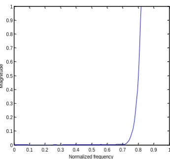
In the high-pass filter designing, the prescribed range of pass-band and stop-pass-band are taken as 0.8π≤ w≤ π and 0≤ w≤0.7π, respectively. The order of the filter is set to 3. The maximum number of iterations for the proposed integrated algorithm is taken as 100. A population of 100 cats is considered with a mixture ratio (MR) of 0.980. The values of MSP, SRD and CDC are set to 5, 0.95 and 0.35, respectively. The maximum number of iterations for the DE algorithm is taken as 35 and the value of the crossover rate (CR) and the mutation factor (fm) are
set equal to 0.85 and 0.25, respectively. The high-pass digital IIR filter model obtained by the proposed algorithm for lower order is given below in Eq. (30).
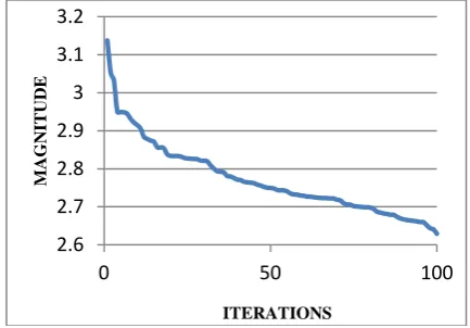
The results obtained by implementing the proposed algorithm for the high-pass digital IIR filter design for order 3 are summarized in Table 3. The frequency response, pole-zero diagrams and the magnitude versus iterations graphs for the high-pass filter are presented in Figure2, Figure 6 and Figure 10, respectively.
A comparison of the obtained results is carried out with the high- pass filter design results given by HGA [7], HTGA [16], TIA [17], Hybrid method [32], Heuristic method [36], PPO [34] and DE [38]. From Table 3, it is observed that the proposed integrated algorithm is capable of producing results that are superior as compared to the results given by other algorithms. Moreover, from Figure 6 it is clear that all the poles lie inside the unit circle, therefore the designed High pass filter is stable and it strictly follows the stability constraints that are imposed during its designing.
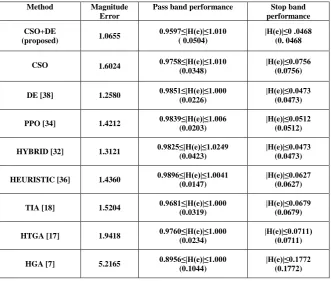
5.1.3 Band-pass filter design
In the band-pass filter designing, the prescribed range of pass-band and stop-pass-band are taken as 0.4π≤ w≤0.6π and 0≤ w≤0.25π, 0.75π≤ w≤ π, respectively. The values of both M and N are taken as 0 and 3, respectively. The maximum number of iterations for the proposed integrated algorithm is taken as 100. A population of 50 cats is considered with a mixture ratio (MR) of 0.50. The values of MSP, SRD and CDC are taken as 5, 0.95 and 0.25, respectively. The maximum number of iterations for the DE algorithm is taken as 35 and the value of the crossover rate (CR) and the mutation factor (fm) are set equal to 0.85 and
0.25, respectively. The band-pass digital IIR filter model obtained by the proposed algorithm for lower order is given below in Eq. (31).
band-pass filter are presented in Figure 3, Figure 7 and Figure 11, respectively.
A comparison of the obtained results is carried out with the band-pass filter design results given by HGA [7], HTGA [16], TIA [17], Hybrid method [32], Heuristic method [36], PPO [34] and DE [38]. From Table 4 it is observed that the proposed integrated algorithm is capable of producing results that are superior as compared to the results given by other algorithms. Moreover, from Figure 7 it is clear that all the poles lie inside the unit circle, therefore the designed band-pass filter is stable and it strictly follows the stability constraints that are imposed during its designing.
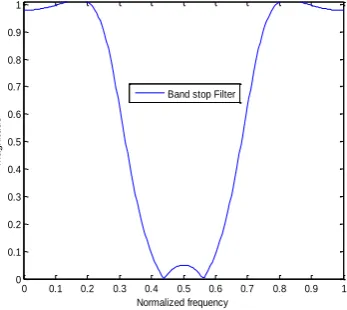
5.1.4 Band-stop filter design
In the band-stop filter designing, the prescribed range of pass-band and stop-pass-band are taken as 0≤ w≤0.25π, 0.75π≤ w≤ π and 0.4π≤ w≤0.6π, respectively. The order of the filter is set to 4. The maximum number of iterations for the proposed integrated algorithm is taken as 100. A population of 50 cats is considered with a mixture ratio (MR) of 0.50. The values of MSP, SRD and CDC are taken as 5, 0.95 and 0.25, respectively. The maximum number of iterations for the DE algorithm is taken as 35 and the
value of the crossover rate (CR) and the mutation factor (fm) are
set equal to 0.85 and 0.25, respectively. The band-stop digital IIR filter model obtained by the proposed algorithm for lower order is given below in Eq. (32).
The results obtained by implementing the proposed algorithm for the band-stop digital IIR filter design for order 4 are summarized in Table 5. The frequency response, pole-zero diagrams and the magnitude versus iterations graphs for band-stop filter are presented in Figure 4, Figure 8 and Figure 12, respectively.
A comparison of the obtained results is carried out with the band-stop filter design results given by HGA [7], HTGA [16], TIA [17], Hybrid method [32], Heuristic method [36], PPO [34] and DE [38]. From Table 5 it is observed that the proposed integrated algorithm is capable of producing results that are superior as compared to the results given by other algorithms. Moreover, from Figure 8 it is clear that all the poles lie inside the unit circle, therefore the designed band-stop filter is stable and it strictly follows the stability constraints that are imposed during its designing.
(29)
(30)
(31)
(32) [image:7.595.324.497.489.650.2]
Figure 4: Frequency response of high-pass filter
0 0.1 0.2 0.3 0.4 0.5 0.6 0.7 0.8 0.9 1 0
0.1 0.2 0.3 0.4 0.5 0.6 0.7 0.8 0.9 1
M
a
g
n
it
u
d
e
Normalized frequency
Low Pass Filter
0 0.1 0.2 0.3 0.4 0.5 0.6 0.7 0.8 0.9 1
0 0.1 0.2 0.3 0.4 0.5 0.6 0.7 0.8 0.9 1
M
a
g
n
it
u
d
e
Normalized frequency
0 0.1 0.2 0.3 0.4 0.5 0.6 0.7 0.8 0.9 1
0 0.1 0.2 0.3 0.4 0.5 0.6 0.7 0.8 0.9 1
M
a
g
n
it
u
d
e
Normalized frequency
Band Pass Filter
0 0.1 0.2 0.3 0.4 0.5 0.6 0.7 0.8 0.9 1
0 0.1 0.2 0.3 0.4 0.5 0.6 0.7 0.8 0.9 1
M
a
g
n
it
u
d
e
Normalized frequency Band stop Filter
-1 -0.5 0 0.5 1
-1 -0.5 0 0.5 1
Real part
Im
a
g
in
a
ry
p
a
rt
Low Pass Filter
-1 -0.5 0 0.5 1
-1 -0.5 0 0.5 1
Real part
Im
a
g
in
a
ry
p
a
rt
High Pass Filter
-1 -0.5 0 0.5 1
-1 -0.5 0 0.5 1
Real part
Im
a
g
in
a
ry
p
a
rt
Band Pass Filter
-1 -0.5 0 0.5 1
-1 -0.5 0 0.5 1
Real part
Im
a
g
in
a
ry
p
a
rt
[image:8.595.313.487.84.239.2]Band Stop Filter Figure 4: Frequency response of band-stop filter Figure 3: Frequency response of band-pass filter
Figure 5: Pole-zero graph of low-pass filter Figure 6: Pole-zero graph of high-pass filter
[image:8.595.72.259.86.241.2]
Figure 9: Magnitude versus Iterations for low-pass filter Figure 10: Magnitude versus Iterations for high-pass filter
Figure 11: Magnitude versus Iterations for band-pass filter Figure 12: Magnitude versus Iterations for band-stop filter
Table 2. Design results for low-pass filter
Method Magnitude
Error Pass band performance Stop band performance
CSO+DE
(proposed) 3.4678
0.8455≤|H(e)|≤1.040 (0.1948)
|H(e)|≤0.1129 (0.1129)
CSO 3.7759 0.9376≤|H(e)|≤1.021
(0.0835)
|H(e)|≤0.1567 (0.1567)
DE [38] 3.5014 0.8838≤|H(e)|≤1.019 (0.1353)
|H(e)|≤0.1505 (0.1505)
PPO [34] 3.6611 0.9178≤|H(e)|≤1.000 (0.0998) |H(e)|≤0.1611 (0.1611)
HYBRID[32] 3.7903 0.9283≤|H(e)|≤1.026 (0.0976)
|H(e)|≤0.1405 (0.1405)
HEURISTIC [36] 4.1145 0.9246≤|H(e)|≤1.011 (0.0871)
|H(e)|≤0.1238 (0.1238)
TIA [18] 3.8157 0.8914≤|H(e)|≤1.000 (0.1086)
|H(e)|≤0.1638 (0.1638)
HTGA [17] 4.2511 0.9000≤|H(e)|≤1.000 (0.0996)
|H(e)|≤0.1247 (0.1247)
HGA [7] 4.3395 0.8870≤|H(e)|≤1.009 (0.1139)
|H(e)|≤0.1802 (0.1802)
3.45
3.5 3.55 3.6 3.65
0 20 40 60 80 100
M
A
GN
IT
U
D
E
ITERATIONS
2.6 2.7 2.8 2.9 3 3.1 3.2
0 50 100
M
A
G
N
ITU
D
E
ITERATIONS
0.3 0.5 0.7 0.9 1.1
0 50 100
M
AG
NIT
UDE
ITERATIONS
2.9 3.1 3.3 3.5 3.7 3.9
0 20 40 60 80 100
M
A
GN
IT
U
D
E
Table 3. Design results for high-pass filter
Method Magnitude
Error Pass band performance Stop band performance
CSO+DE
(proposed) 2.7119
[image:10.595.133.465.390.671.2]0.9396≤|H(e)|≤ 1.009 (0.0695)
|H(e)|≤0.0499 (0.0499)
CSO 4.4900 0.8299≤|H(e)|≤1.025
(0.1954)
|H(e)|≤0.1285 (0.1285)
DE [38] 2.8960 0.8955≤|H(e)|≤1.014 (0.1188)
|H(e)|≤0.1100 (0.1505)
PPO [34] 3.9332 0.9401≤|H(e)|≤1.0010 (0.0717)
|H(e)|≤0.1692 (0.1692)
HYBRID [32] 3.9724 0.9625≤|H(e)|≤1.0265
(0.0639) |H(e)|≤0.1536
(0.1536)
HEURISTIC [36] 4.6635 0.9584≤|H(e)|≤1.0080
(0.0504) |H(e)|≤0.1477
(0.1477)
TIA [18] 4.1819 0.9229≤|H(e)|≤1.000 (0.0771)
|H(e)|≤0.1424 (0.1424)
HTGA [17] 4.8372 0.9460≤|H(e)|≤1.000 (0.0540) |H(e)|≤0.1457 (0.1457)
HGA [7] 14.5.78 0.9224≤|H(e)|≤1.001 (0.0779)
|H(e)|≤0.1819 (0.1819)
Table 4. Design results for band-pass filter
Method Magnitude Error
Pass band performance Stop band performance
CSO+DE
(proposed) 1.0655
0.9597≤|H(e)|≤1.010 ( 0.0504)
|H(e)|≤0 .0468 (0. 0468
CSO 1.6024 0.9758≤|H(e)|≤1.010
(0.0348)
|H(e)|≤0.0756 (0.0756)
DE [38] 1.2580 0.9851≤|H(e)|≤1.000 (0.0226)
|H(e)|≤0.0473 (0.0473)
PPO [34] 1.4212 0.9839≤|H(e)|≤1.006 (0.0203)
|H(e)|≤0.0512 (0.0512)
HYBRID [32] 1.3121 0.9825≤|H(e)|≤1.0249 (0.0423)
|H(e)|≤0.0473 (0.0473)
HEURISTIC [36] 1.4360 0.9896≤|H(e)|≤1.0041 (0.0147)
|H(e)|≤0.0627 (0.0627)
TIA [18] 1.5204 0.9681≤|H(e)|≤1.000 (0.0319)
|H(e)|≤0.0679 (0.0679)
HTGA [17]
1.9418 0.9760≤|H(e)|≤1.000 (0.0234)
|H(e)|≤0.0711) (0.0711)
HGA [7] 5.2165 0.8956≤|H(e)|≤1.000 (0.1044)
Table 5. Design results for band-stop filter
5.2 Higher order digital IIR filter design
For designing higher order digital IIR filter, 200 equally spaced points are set within the frequency domain [0, π]. The order of the digital IIR filter is given as M+2N; where M and N denotes the number of filter coefficients. In the proposed method the value of the order of the digital IIR filter for the LP, HP, BP and BS filters has been varied ranging from 1 to 30 by varying the values of M and N. In other words, the order of the filter is not kept constant. The objective of the optimization problem is to minimize the absolute error (i.e., L1-norm) of magnitude
response subject to the stability constraints given by Eq. (9.1) - Eq. (9.5) under the prescribed design conditions given in Table 1.
For higher order digital IIR low-pass filter, the values of M and N are varied. The maximum number of iterations for the proposed integrated algorithm has been set to 100. A population of 100 cats is considered with a mixture ratio (MR) of 0.755. The values of MSP, SRD and CDC are taken as 20, 0.25 and 0.80, respectively. The maximum number of iterations for the DE algorithm is taken as 35 and the value of the crossover rate (CR) and the mutation factor (fm) are set equal to
0.85 and 0.25, respectively. The proposed algorithm shows the capability to design a stable low-pass filter with values of M and N equal to 1 and 10, respectively i.e. the order of the filter is 21. This designed filter with an order of 21 showed better magnitude approximation error over all other orders. The magnitude approximation error and the pass-band and stop-band ripple magnitudes for the higher order low-pass are
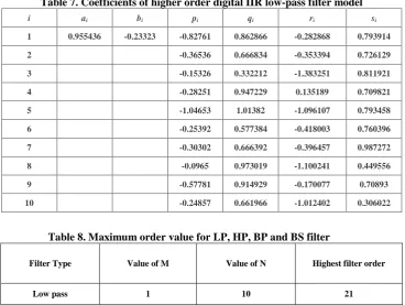
summed up in Table 6. The coefficients of the design model obtained for the higher order digital IIR low-pass filter are shown in Table 7. The frequency response and pole-zero diagrams for the higher order digital low-pass filter are given in Fig. 13 and Fig. 14, respectively. As all the poles lie inside the unit circle, therefore the designed high order low-pass filter is stable and it strictly follows the stability constraints that are imposed during its designing.
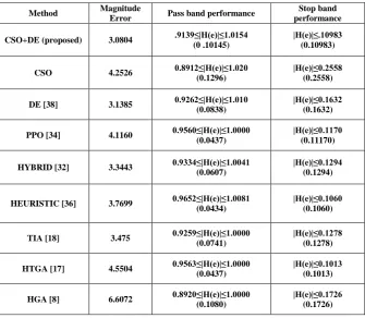
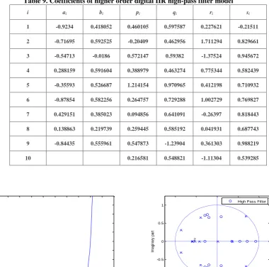
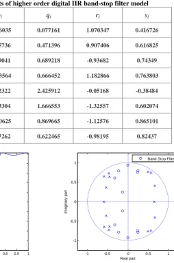
A similar approach has been followed for designing the higher order digital IIR high-pass, band-pass and band-stop filters. The maximum value of order for the digital IIR LP, HP, BP, and BS filters for which the implemented algorithm shows competitive results is given in Table 8. The magnitude approximation error and the pass-band and stop-band ripple magnitudes for the higher order high-pass, band-pass and band-stop filters are summed up in Table 6. The coefficients of the design model obtained for the higher order digital IIR high-pass, band-pass and band-stop filters are given in Table 9, Table 10 and Table 11, respectively. The frequency response and pole-zero diagrams for the higher order digital high-pass, band-pass and band-stop filters are given in Fig. 15- Fig. 20. In each case all the poles lie inside the unit circle, therefore the designed high order high-pass, band-pass and band-stop filters are stable and strictly follow the stability constraints that are imposed during their designing.
Method Magnitude
Error Pass band performance
Stop band performance
[image:11.595.131.467.88.380.2]CSO+DE (proposed) 3.0804 .9139≤|H(e)|≤1.0154 (0 .10145)
|H(e)|≤.10983 (0.10983)
CSO 4.2526 0.8912≤|H(e)|≤1.020
(0.1296)
|H(e)|≤0.2558 (0.2558)
DE [38] 3.1385 0.9262≤|H(e)|≤1.010 (0.0838)
|H(e)|≤0.1632 (0.1632)
PPO [34] 4.1160 0.9560≤|H(e)|≤1.0000 (0.0437)
|H(e)|≤0.1170 (0.11170)
HYBRID [32] 3.3443 0.9334≤|H(e)|≤1.0041 (0.0607)
|H(e)|≤0.1294 (0.1294)
HEURISTIC [36] 3.7699 0.9652≤|H(e)|≤1.0081 (0.0434)
|H(e)|≤0.1060 (0.1060)
TIA [18] 3.475 0.9259≤|H(e)|≤1.0000 (0.0741)
|H(e)|≤0.1278 (0.1278)
HTGA [17]
4.5504 0.9563≤|H(e)|≤1.0000 (0.0437)
|H(e)|≤0.1013 (0.1013)
HGA [8]
6.6072 0.8920≤|H(e)|≤1.0000 (0.1080)
Table 6. Design results for LP, HP, BP and BS filters for higher orders
Filter Magnitude
Error Pass band performance Stop band performance Low pass 0.4415 .9736≤|H(e)|≤ 1.0025
[image:12.595.114.483.404.681.2] [image:12.595.113.483.404.599.2](.0289)
|H(e)|≤ .0165 (.0165)
High pass 1.3011 .9566≤|H(e)|≤1.0035 (.0469)
|H(e)|≤ .0365 (.0365) Band pass 1.4050 0.8983≤|H(e)|≤1.0259
(0.1276)
|H(e)|≤0.0558 (0.0558) Band stop 1.5962 0.9383≤|H(e)|≤1.0369
(0.0987)
|H(e)|≤0.0058 (0.0058)
Figure 13: Frequency response of low-pass filter Figure 14: Pole-zero graph of low-pass filter
Table 7. Coefficients of higher order digital IIR low-pass filter model
i ai bi pi qi ri si
1 0.955436 -0.23323 -0.82761 0.862866 -0.282868 0.793914
2 -0.36536 0.666834 -0.353394 0.726129
3 -0.15326 0.332212 -1.383251 0.811921
4 -0.28251 0.947229 0.135189 0.709821
5 -1.04653 1.01382 -1.096107 0.793458
6 -0.25392 0.577384 -0.418003 0.760396
7 -0.30302 0.666392 -0.396457 0.987272
8 -0.0965 0.973019 -1.100241 0.449556
9 -0.57781 0.914929 -0.170077 0.70893
10 -0.24857 0.661966 -1.012402 0.306022
Table 8. Maximum order value for LP, HP, BP and BS filter
Filter Type Value of M Value of N Highest filter order
Low pass 1 10 21
High pass 9 10 29
Band pass 8 8 24
Band stop 0 8 16
0 0.1 0.2 0.3 0.4 0.5 0.6 0.7 0.8 0.9 1
0 0.1 0.2 0.3 0.4 0.5 0.6 0.7 0.8 0.9 1
M
a
g
n
it
u
d
e
Normalized frequency
Low Pass Filter
-1 -0.5 0 0.5 1
-1 -0.5 0 0.5 1
Real part
Im
a
g
in
a
ry
p
a
rt
Table 9. Coefficients of higher order digital IIR high-pass filter model
i ai bi pi qi ri si
1 -0.9234 0.418052 0.460105 0.597587 0.227621 -0.21511
2 -0.71695 0.592525 -0.20409 0.462956 1.711294 0.829661
3 -0.54713 -0.0186 0.572147 0.59382 -1.37524 0.945672
4 0.288159 0.591604 0.388979 0.463274 0.775344 0.582439
5 -0.35593 0.526687 1.214154 0.970965 0.412198 0.710932
6 -0.87854 0.582256 0.264757 0.729288 1.002729 0.769827
7 0.429151 0.385023 0.094856 0.641091 -0.26397 0.818443
8 0.138863 0.219739 0.259445 0.585192 0.041931 0.687743
9 -0.84435 0.555961 0.547873 -1.23904 0.361303 0.988219
[image:13.595.102.483.77.453.2] [image:13.595.119.482.531.732.2]10 0.216581 0.548821 -1.11304 0.539285
Figure 15: Frequency response of high-pass filter Figure 16: Pole-zero graph of high-pass filter
Table 10. Coefficients of higher order digital IIR band-pass filter model
i ai bi pi qi ri si
1 -0.01612 -0.82934 -0.035871 -0.03587 -0.00142 0.333975
2 -0.00057 -0.48702 0.000176 -0.72184 -0.16715 0.240474
3 0.001655 -0.39692 0.000625 0.545119 0.3156 0.637425
4 -0.00074 0.205631 0.014481 0.017047 -0.00127 0.237155
5 -0.32179 0.859644 -0.000071 -0.88273 -0.63178 0.431595
6 0.485594 0.609457 0.001495 -0.31395 0.879371 0.953247
7 0.268998 -0.89744 -0.013903 -1.62367 -0.06631 0.304196
8 -0.02625 0.588891 -0.000261 -0.83095 -0.48391 0.629734
0 0.1 0.2 0.3 0.4 0.5 0.6 0.7 0.8 0.9 1
0 0.1 0.2 0.3 0.4 0.5 0.6 0.7 0.8 0.9 1
M
a
g
n
it
u
d
e
Normalized frequency
-1 -0.5 0 0.5 1
-1 -0.5 0 0.5 1
2
Real part
Im
ag
in
ar
y
pa
rt
Figure 17: Frequency response of band-pass filter Figure 18: Pole-zero graph of band-pass filter
Table 11. Coefficients of higher order digital IIR band-stop filter model
i pi qi ri si
1 0.276035 0.077161 1.070347 0.416726
2 -0.65736 0.471396 0.907406 0.616825
3 -0.49041 0.689218 -0.93682 0.74349
4 0.463564 0.666452 1.182866 0.763803
5 -0.42322 2.425912 -0.05168 -0.38484
6 -0.23304 1.666553 -1.32557 0.602074
7 0.010625 0.869665 -1.12576 0.865101
[image:14.595.79.490.117.640.2]8 -0.47262 0.622465 -0.98195 0.82437
Figure 19: Frequency response of band-stop filter Figure 20: Pole-zero graph of band-stop filter
5.3 Robustness of the Proposed Method
In order to check the robustness of the proposed algorithm to achieve global design for order 3 LP, order 3 HP, order 6 BP and order 4 BS filter design, 100 independent trial runs have been given with random seed numbers for each case and the variations in the magnitude response has been observed. The maximum value, minimum value, average value and standard deviation in magnitude approximation error are given in Table 12. From the results it can be observed that for each case, the
standard deviation is very small which indicates the robustness of the designed algorithm.
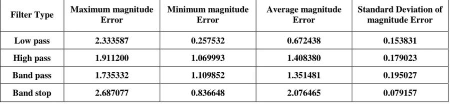
A similar approach has been followed to check the robustness of the proposed algorithm to achieve global design for the design of higher order digital IIR filters. In this case too, for each filter, 100 independent trial runs are carried out. The variation in the magnitude response of all the filters has been studied. The maximum value, minimum value, average value and standard deviation of the magnitude response error are given in Table 13. The results obtained depict that for higher
0 0.1 0.2 0.3 0.4 0.5 0.6 0.7 0.8 0.9 1
0 0.1 0.2 0.3 0.4 0.5 0.6 0.7 0.8 0.9 1
M
a
g
n
it
u
d
e
Normalized frequency
Band Pass Filter
-1 -0.5 0 0.5 1
-1 -0.5 0 0.5 1
Real part
Im
ag
in
ar
y
pa
rt
Band Pass Filter
0 0.1 0.2 0.3 0.4 0.5 0.6 0.7 0.8 0.9 1 0
0.1 0.2 0.3 0.4 0.5 0.6 0.7 0.8 0.9 1
M
a
g
n
it
u
d
e
Normalized frequency Band Stop Filter
-1 -0.5 0 0.5 1
-1 -0.5 0 0.5 1
Real part
Im
a
g
in
a
ry
p
a
rt
[image:14.595.223.478.253.639.2]order digital IIR LP, HP, BP and BS filters the standard deviation is very small, which proves the robustness of the
[image:15.595.72.526.118.228.2]proposed algorithm again.
Table 12: Maximum, Minimum, Average values and Standard deviation of Magnitude error for lower filter orders
Filter Type Maximum magnitude Error
Minimum magnitude Error
Average magnitude Error
Standard Deviation of magnitude Error
Low pass 3.644905 3.465051 3.516012 0.003375 High pass 3.138020 2.629057 2.77214 0.043194 Band pass 1.084589 0.431594 0.848758 0.026284 Band stop 3.770113 3.036197 3.128349 0.017186
Table 13: Maximum, Minimum, Average values and Standard deviation of Magnitude error for higher filter orders
Filter Type Maximum magnitude Error
Minimum magnitude Error
Average magnitude Error
Standard Deviation of magnitude Error
Low pass 2.333587 0.257532 0.672438 0.153831 High pass 1.911200 1.069993 1.408380 0.179023 Band pass 1.735332 1.109852 1.351481 0.195027 Band stop 2.687077 0.836648 2.076465 0.079157
6. CONCLUSION
Although the digital IIR filter design is an active area of research, most of the population based optimization algorithms face difficulties like search stagnation, slow convergence etc. This paper proposes an integrated cat swarm and differential evolution algorithm for the optimal design of digital IIR LP, HP, BP and BS filters. The performance assessment of the proposed integrated algorithm is carried out by comparing the obtained results with other well known algorithms. From the results obtained it is clear that the proposed algorithm is very much feasible for the designing of digital IIR filters under prescribed design conditions. The algorithm not only outperforms other proposed algorithms for minimum value of the order for the LP, HP, BP, and BS filters but is also capable of designing filters with even higher order values. Further, the proposed algorithm for designing the LP, HP, BP and BS filter, allows each filter to be designed independently. Parameter tuning is still a potential area for further research. The proposed algorithm has the capability to search the solution locally as well as globally and takes a start with good population.
7. ACKNOWLEDGEMENTS
This research paper is made possible through the help and support from parents, teachers and friends. I dedicate my acknowledgement of gratitude towards my guide ‘Dr. J. S. Dhillon’ for his kind support, encouragement and advice on every step. I thank my parents and family, without whose financial and moral support, this work would not have been materialized
8. REFERENCES
[1] I. Jury, Theory and Application of the Z-Transform Method, New York: Wiley, 1964.
[2] S.K. Mitra and J.F. Kaiser, Handbook for Digital Signal Processing, Wiley, New York, 1993.
[3] J. Kennedy and R. Eberhart, “Particle Swarm Optimization,” IEEE International Conference on Neural
Networks, Piscataway, New Jersey, U.S.A, vol. 4, pp. 1942-1948, 1995.
[4] R. Storm and K. Prince, “Differential evolution-A Simple and Efficient Heurist for Global Optimization over Continuous Spaces,” University of California, Berkeley, International Computational Sciences Institute, Berkeley, March 1995.
[5] J.H. Li and F.L. Yin, “Genetic Optimization Algorithm for Designing IIR Digital Filters,” Journal of China Institute of Communications, vol. 17, pp. 1–7, 1996.
[6] J.M. Renders and S.P. Flasse, “Hybrid Methods Using Genetic Algorithms for Global Optimization,” IEEE Transactions on Systems, Man, and Cybernetics-Part B, vol. 26, no. 2, pp. 243-258, April 1996.
[7] K.S. Tang, K.F. Man, S. Kwong and Z.F. Liu, “Design and Optimization of IIR Filter Structure using Hierarchical Genetic Algorithms,” IEEE Transaction on Industrial Electronics, vol. 45, no. 3, pp. 481–487, June 1998. [8] K. Deb, Multi-Objective Optimization Using Evolutionary
Algorithms, Wiley, New York, 2001.
[9] A. Silva, A. Neves and E. Costa, “An Empirical comparison of Particle Swarm and Predator Prey Optimization,” Proceedings of Irish International Conference on Artificial Intelligence and Cognitive Science, vol. 24, no.64, pp 103-110, 2002.
[10]Y. S. Ong and A. J. Keane, “A Domain Knowledge based Search Advisor for Design Problem solving environments,” Engineering Application and Artificial Intelligence, vol. 15, no. 1, pp. 105–116, 2002.
[image:15.595.73.524.255.363.2][12]N. Karaboga, A. Kalinli, and D. Karaboga, “Designing IIR Filters using Ant Colony Optimization Algorithm,” Journal of Engineering Applications of Artificial Intelligence, vol. 17, no. 3, pp. 301–309, April 2004. [13]A. Kalinli and N. Karaboga, “A New Method for Adaptive
IIR Filter Design Based On Tabu Search Algorithm,” International Journal of Electronics and Communication (AEÜ), vol. 59, no. 2, pp. 111–117, 2005.
[14]X. Li, “Efficient Differential Evolution using Speciation for Multimodal Function Optimization,” Proceedings of International Conference on Evolutionary Computation, , pp. 873–880, 2005.
[15]Y. S. Ong, M. H. Lim, N. Zhu, and K. W. Wong, “Classification of Adaptive Memetic Algorithms: A comparative study,” IEEE Transaction on System Man and Cybernatics Part B: Cybernatics, vol. 36, no. 1, pp. 141– 152, Feb. 2006.
[16]Jinn-Tsong Tsai, Jyh-Horng Chou and Tung-Kuan Liu, “Optimal Design of Digital IIR filters by using Hybrid Taguchi Genetic Algorithm,” IEEE Transactions on Industrial Electronics, vol. 53, no. 3, pp. 867–879, June 2006.
[17]Jinn-Tsong Tsai and Jyh-Horng, “Optimal Design of Digital IIR Filters using an Improved Immune Algorithm,” IEEE transactions on Signal Processing, vol. 54, no. 12, pp. 4582–4596, December 2006.
[18]S. C. Chu and P. W.Tsai, “Computational Intelligence based on the Behavior of Cat,” International Journal of Innovative computing, Information and Control, vol. 3, no. 1, pp.163-173, 2007.
[19]Y. Yu and Y. Xinjie, “Cooperative co-evolutionary Genetic Algorithm for Digital IIR Filter Design,” IEEE Transactions on Industrial Electronics, vol. 54, no. 3, pp. 1311–1318, June 2007.
[20]Rahnamayan, H.R. Tizhoosh and M.A. Salama, “Opposition based Differential Evolution,” IEEE Transactions on Evolutionary Computations, vol. 12, no.1, pp 64-79, February 2008.
[21]V.Y Del, G.K. Venayagamoorthy, S. Mohagheghi, J.C.G. Hernandez and R. Harely, “Particle Swarm Optimization: Basic Concepts, Variants and Applications in Power Systems,” IEEE Transactions on Evolutionary Computation, vol. 12, no. 2, pp 171-195, 2008.
[22]N. Noman and H. Iba, “Accelerating Differential Evolution Using an Adaptive Local Search,” IEEE Transactions on Evolutionary Computation, vol. 12, no 1, pp 107-125, February 2008.
[23]Sum-Im, G.A. Taylor, M.R. Irving and Y.H. Song, “Differential Evolution Algorithm for Static Multistage Transmission Expansion Planning,” IET Generation, Transmission and Distribution, vol. 3, no. 4, pp 365-384, 2009.
[24]Aimin Jiang and Hon Keung Kwan, “IIR Digital Filter Design with New Stability Constraint based on Argument Principle,” IEEE Transactions on Circuit and Systems-I, vol. 56, no. 3, pp. 583–593, March 2009.
[25]A.K. Qin, V.L. Huang and P.N. Sugathan, “Differential Evaluation Algorithm With Strategy Adapter for Global Numerical Optimization,” IEEE Transactions on
Evolutionary Computation, vol. 13, no. 2,pp 398-417, April 2009.
[26]S. Chattopadhyay, S. K. Sanyal and A. Chandra, “Design of FIR Filter using Differential Evolution Optimization and is Effect as a Pulse Shaping Filter In a QPSK Modulated System,” International Journal of Computer Science and Network Security, vol. 10, no. 1, pp. 313-321, January 2010.
[27]D. Chaohua , W. Chen and Y. Zhu, “Seeker Optimization Algorithm for Digital IIR Filter Design,” IEEE Transactions on Industrial Electronics, vol. 57, no. 5, pp. 1710-1718, May 2010.
[28]Proakis, J.G., Digital signal processing, Prentice-Hall International. Inc., New Jersey, (2010).
[29]S. Das and P.N. Suganthan, “Differential Evolution: A Survey of the State-of-the-Art, “IEEE Transactions on Evolutionary Computation,” vol. 15, no. 1, pp. 4-31, February 2011.
[30]G. Panda, P.M. Pradhan and B. Majhi, “IIR System Identification Using Cat Swarm Optimization,” Expert Systems with Applications, vol. 38, no. 10, pp. 12671-12683, September 2011.
[31]D. P. Kothari and J. S. Dhillon, Power system Optimization, Prentice Hall of India, 2nd Edition, New Delhi, (2011).
[32]R. Kaur, M.S. Patterh, J.S. Dhillon, “Design of Optimal L1
Stable IIR Digital Filter using Hybrid Optimization Algorithm,” International Journal of Computer Applications, vol. 38, no 2 ,pp 27-32, January 2012. [33]Pei-Wei Tsai, Jeng-Shyang Pan, Shyi-Ming Chen and
Bin-Yih Lio, “Enhanced Parallel Cat Swarm Optimization based on the Taguchi method,” Expert Systems with Applications, vol. 39, no. 10, pp. 6309-6319, 2012. [34]B. Singh, J.S Dhillon, Y. S. Brar, “Design of Digital IIR
filter: A Comparison,” International journal of Electrical, Electronics and Telecommunication Engineering, vol. 44, no. 1, pp. 1108-1121, February 2012.
[35]P. M. Mohan and G. Panda, “Solving Multiobjective Problems using Cat Swarm Optimization,” Expert Systems with Applications, vol. 39, no. 10, pp. 2956-2964, 2012. [36]R. Kaur, M.S Patterh, J.S Dhillon and D. Singh, “Heuristic
search method for digital IIR filters design,” Wseas Transactions on Signal Processing, vol. 8, pp. 121-134, July 2012.
[37]Zhi-Hui Wang, Chin-Chen Chang and Ming-Chu Li, “Optimizing Least-Significant-Bit Substitution using Cat Swarm Optimization Strategy,” Information Sciences, vol. 192, no., pp. 98-108, 2012.
[38]B. Singh, J.S Dhillon and Y. S. Brar, “A Hybrid Differential Evolution Method for the Design of IIR Digital Filter,” International Journal on Signal and Image Processing, vol. 4, no. 1, pp. 1-10, January 2013.