Munich Personal RePEc Archive
The Costs to Consumers of a
Depreciated Conversion Rate to the Euro
Marques, Luis B
Johns Hopkins University - SAIS
August 2007
The Costs to Consumers of a Depreciated Conversion
Rate to the Euro
∗
Luis Marques
August 12, 2007
Abstract
This paper measures the welfare cost to consumers of the bloc of Central and
Eastern European Countries (CEEC), plus Malta and Cyprus, of choosing a
de-preciated conversion rate when joining the European Monetary Union. For this, I
present and solve an appropriately calibrated small open economy model where a
euro-denominated bond and the equity on a traded goods sector are traded
inter-nationally. I show that the cost of depreciating the domestic currency against the
euro by 20%, at the time of joining the European Monetary Union, entails a cost of
approximately 1.65% in terms of lost lifetime utility (measured in equivalent units
of consumption).
JEL classification: F31, F41, F47.
Keywords: trade effect, valuation effect, wealth effect, exchange rate.
1
Introduction
Since 2004, several countries from Central and Eastern Europe, as well as Malta and
Cyprus, have joined the European Union (EU). One of the conditions for the accession was
the commitment to join the European Monetary Union (EMU) and to drop its national
currencies in favor of the euro sometime in the future. For this to be accomplished, the
new members of the EU have to fulfil several requirements regarding macroeconomic
stability, namely maintaining a managed float with the euro.1
However, several authors within the equilibrium exchange rate literature as well as
advisors to policymakers have argued for a sizeable overvaluation of many of the
curren-cies from the CEEC.2
The results presented by R¨ahn (2003), Bul´ı˘r and ˘Smi´ıdkov´a (2005),
and ´Egertet al. (2005), to name a few, seem to indicate that prior to entry to the EMU,
the accession countries should depreciate their currencies as a way of preserving their
competitiveness and smoothing the adjustment path.3 Schadler et al. (2005), noting
that these estimates are indeed very imprecise, argue that although there was no sign
of significant over or undervaluation of the currencies of these countries as late as 2002,
due to a perceived asymmetry between the risks of an overvaluation and the risks of an
1
Aspiring members to the EMU must be members for two years to the Exchange Rate Mechanism (mark 2) where currencies are allowed to float against the euro within a±15% band. Additionally, at the time of entry they must show: (1) a fiscal deficit below 3 percent of GDP and public debt of no more than 60 percent of GDP; (2) inflation rates not in excess of the average inflation rates in the EMU countries with the best price stability record by more than 1.5 percent points; and (3) long-term nominal interest rates not exceeding the average of the three preceding countries by more than 2 percentage points. See Schadleret al. (2005) for details.
2
One problem with the equilibrium exchange rate literature is that its results seem to be very de-pendent on the chosen model specification and estimation technique. Rawdanowicz (2006) also raises concerns over this being the right set of methodologies to choose a conversion rate to the euro as it assumes the economy to be at or approaching some appropriately defined internal and external equilib-rium. This is clearly not the case for these transition economies and is not contemplated in the model presented and solved ahead in this paper.
3
undervaluation at the time of entry to EMU, it would be advisable to choose a parity at
the weak end of the equilibrium range.
This concern has found its way to the press, as Christopher Swann noted, in 2002, in
theFinancial Times: “Authorities in the Czech Republic and Hungary have already balked
at a further rise of their exchange rates. Their sights may now turn to containing currency
strength ahead of entering an exchange rate mechanism. With Germany suffering from
having joined the euro at an uncompetitive rate, there would be resistance to any attempts
by prospective members to depreciate their currencies shortly before locking into the euro.”
However, it is not at all clear that such a permanent depreciation is a positive thing and
it surely entails costs.
The purpose of this paper is to quantify the costs accruing to consumers of Central
and Eastern European countries of having a depreciated conversion rate for their domestic
currencies when joining the EMU. This event is represented as a permanent shock to the
exchange rate and not as a decision variable. The reason for this is that joining the EMU
is not entirely (not even mostly) under the CEEC’s control. In fact, although countries
outside the EMU do have something to say as to when to join the Euro Area4
, the first
and last word on this falls with its current members.
The costs of a permanent depreciation of a currency come from two sources: a trade
effect and an asset effect. The trade effect means that the relative price of imports
increases. The asset effect includes a valuation effect and a wealth effect. The valuation
effect means that, at impact, a depreciation will make net foreign assets more valuable
in terms of the domestic currency and consumption goods. Tille (2005) looks at a dollar
depreciation from the US consumer perspective and argues for a positive and very large
valuation effect that could overturn the negative impact of the increased relative price
of imports. However, as follows from Marques (2007), if financial assets are traded
4
internationally, a depreciation of the currencies of the CEEC against the euro means
that these will be relatively poorer and that a portfolio rebalancing effect will be set in
motion. The outcome is that the CEEC will be left with a smaller fraction of total claims
on future dividends. Furthermore, since these countries, contrary to the US, do not have
the privilege of borrowing from foreign creditors in their own currency, a depreciation
causes a transfer of wealth from domestic debtors to foreign creditors.
The work in this paper relates to Mendoza (2001) where the impact of a dollarization
in an emerging market economy is measured when there are endogenously binding credit
constraints and the stabilization policy has imperfect credibility. Unlike Mendoza (2001),
I have exogenous constraints on borrowing and short selling, by means of convex
trans-action costs. Additionally, I assume no money holdings but have equity and bonds being
traded across borders. Finally, Mendoza (2001) models dollarization as an exogenous
drop in the probability of a depreciation occurring whereas I treat it is as an absorbing
state which agents are aware of. Thus, while Mendoza compares two economies with
different probability distributions, I solve for a model where the chance of an exogenous
regime change is part of the information set.
Cooley and Quadrini (2001) look at the issue of dollarization and find substantial
costs for Mexico: almost 0.5% of annual consumption. In that paper, the cost is coming
from Mexico no longer being able to choose its inflation rate optimally after dropping
its currency. Higher inflation and nominal interest rates with monetary independence
translate into a real currency appreciation, which is welfare improving through the trade
channel. This mechanism is, to some extent, analogous to what I find in the current
work: a nominal and permanent currency depreciation translates into a real depreciation
because of price rigidity in the tradable sector, which in turns affects negatively
con-sumers through a trade effect. However, Cooley and Quadrini abstract from asset trade
In the next section, I present a simple model of a small open economy with
interna-tionally traded equity and debt. In Section 3, I present the calibration and the method
used to solve the model. I discuss the results obtained for three simulated experiments
where the CEEC economy is allowed to join the EMU at an uncertain or certain date, at
an appreciated or a depreciated rate, or even not at all, in Section 4. Section 5 concludes.
2
Model with Optimal Portfolio Choice
In this model there are two economies: a small open economy similar to a Central and
Eastern European Country (CEEC) and a large economy that should represent the Euro
Area (EU). The CEEC is assumed to have a domestic currency, while the EU has the euro
as its currency, which serve as numeraires. The nominal exchange rate of this domestic
currency with the EU is given by St and, as in Marques (2007), is exogenously defined.
The small open economy includes two sectors: a traded goods sector and a nontraded
goods sector. The tradable goods sector is composed of two goods: a domestic or CEEC
traded good and a foreign traded good. The CEEC is assumed to have a stochastic
endowment of the domestic traded good,Dt, but has to import from the EU any amount
it wants to consume of the foreign good. The EU is assumed to be able to supply any
quantity of both goods, domestic and foreign, at given prices, P1t and P2t, respectively.
These prices, too, are exogenously set and assumed to be rigid so that a changes in the
nominal exchange rate translate into changes in the terms of trade. This is a required
condition for the existence of welfare implications coming from the trade channel.
The assumption of endogenous production of tradables, not pursued here, is certainly
not innocuous as in a stationary setting it means that a permanent depreciation causes
a permanent competitiveness gain. However, this is no longer true in a production
depreciation. For this reason, it is appropriate to consider the stochastic endowment
setting for tradables in a model without growth.
In a small open economy, exchange rate movements cause important interactions
between the output of tradables and nontradables, and work effort, which do not arise
if one assumes stochastic endowments for both sectors. To include production in the
nontradable goods sector is therefore an acceptable assumption.
The nontradable goods sector is a competitive industry with a large number of
iden-tical firms. These firms demand domestic labor , Hdt, to produce the nontradable good,
YN t, in order to maximize profits in units of the domestic traded good. No capital
accu-mulation is assumed. Furthermore, there is no technological progress and the model is
fully stationary. The firms choose Hdt to maximize
Πt=PN tYN t−WtHdt (1)
subject to
YN t =AtHtγ (2)
given PN t and Wt, the price of nontradables and the wage rate, respectively. In (2), At
is a stochastic technology shock. Profit maximization yields
γYN t/Hdt−Wt= 0. (3)
On the consumption side, there is a representative consumer from each economy,
but the preferences and optimization problem are only explicitly stated for the CEEC
consumer. The representative agent from the EU holds a fraction of the CEEC’s equity
on its tradable goods sector, θ∗
CEEC tradable equity such that it amounts to a constant portfolio share:
a∗t ≡
Qtθt∗+1 StΩ∗t
=a∗, (4)
where Qt is the price of the equity in the CEEC expressed in domestic currency. The
Euro Area’s total portfolio wealth (in euros), Ω∗
t, is assumed to evolve according to an
exogenous stochastic process. The assumption of a constant share for the CEEC equity on
the European portfolio is reasonable as data from the European Central Bank (ECB) on
the ratio of the international investment position in equity to the total stock of financial
assets of households of the Euro Area shows that it can be reasonably approximated by
constant fraction.
The CEEC’s representative agent consumes the two traded goods (domestic and
for-eign) and one nontraded good, in amounts C1t, C2t, and CN t, respectively. It owns a
fraction θt of the equity on the domestic traded good, and it sells its labor to local firms
producing the nontradable good. It also owns the firms producing the nontradable good
and receives the optimal profits, Π∗
t. Following Stockman and Dellas (1989), it is assumed
that the equity on the firms that produce the non traded good is entirely domestically
owned. To keep the model simple, it is assumed that the CEEC investor chooses not to
own any foreign equity.
This consumers’ problem is:
max
{C1t,C2t,CN t,θt+1,Bt+1,ht}
E0 ∞
X
t=1
subject to
P1tC1t+StP2tC2t+PN tCN t+Qθtθt+1+Bt+1 ≤(Qt+Dt)θt+ (1 +rt)Bt
+WtHst+ Π∗t +T Ct (5)
where
U(C1t, C2t, CN t, Hst) = ³
Ct− Hdt1+ρ
1+ρ ´1−σ
1−σ Ct ≡ (λ1+µC−
µ
T t + (1−λ)
1+µC−µ N t)
−1
µ
CT t ≡ µ
C1t
α
¶αµ
C2t
1−α
¶1−α
,
given prices Qt, PN t, Wt, and per capita aggregate asset holdings ˜Bt,θ˜t.
The consumer pays convex transaction costs on bonds and equity:
T Ct ≡ψ2St(Bt)2+ψ3Qt(θt+1−θt)2. (6)
This condition is imposed to ensure that net foreign assets are stationary, as in Mendoza
and Uribe (2000) and Schmitt-Grohe and Uribe (2003)5 .
As it is apparent from (5), it is assumed that the CEEC can only hold euro
de-nominated bonds. Although a simplification, it is not too far from reality: Lane and
Miles-Ferreti (2006b) calculate the share of foreign currency denominated issues in total
international bond issues by the CEEC, in 2005, to range between 92% for Slovakia and
100% for Estonia, Hungary, Latvia, and Poland. According to the same source, the share
5
This produces the same results as a debt elastic interest rate:
rt=r∗+p( ˜Bt),
of euro denominated issues for this group of countries is between 66% for Hungary and
100% for Latvia6 .
The way labor effort enters the instant utility index is taken from Greenwood et al.
(1988), which is widely used in small open economy models (take Schmitt-Groh´e and
Uribe (2003), for instance). In this formulation, adopted for computational convenience,
the labor effort choice is independent of the intertemporal consumption-savings choice.
The market clearing conditions are:
• in the labor market
Hst =Hdt (7)
• in the equity market
θt+θt∗ = 1 (8)
• in the nontraded goods market
CN t=YN t. (9)
The exchange rate is assumed to follow a Markov chain with four possible states: an
appreciated value for one period, a depreciated value for one period, a depreciated value
forever, and an appreciated value forever. This means that the CEEC can join the EMU
at two possible conversion rates and that joining or not is not something under their
control. All other exogenous shocks (Dt, At, and Ω∗t) are assumed to be Markov chains
derived from AR(1) processes with two possible values each - a high and low one.
Finally, since this is a representative agent economy, consistency conditions are
im-6
posed over individual and per capita aggregate bond and equity holdings:
˜
Bt =Btand ˜θt=θt. (10)
Definition 1 an Equilibrium in this economy is a set of allocations{C1t, C2t, CN t, θt+1, Bt+1, ht}∞t=1, aggregate asset holdings {B˜t+1,θ˜t+1}t∞=1 and prices {Qt, PN t, Wt} such that consumers
solve their utility maximization problem, markets clear, and consistency between
indi-vidual and per capita aggregate asset holdings is verified, given A0, D0,Ω∗0, S0, θ0 and B0.
The forcing variables are {Dt, At,Ω∗t, St}, the aggregate co-states are ˜Bt and ˜θt and
the individual co-states areBtandθt. In this economy there areN = 24×2 = 32 discrete
states. We have then to solve this problem over a grid of M points for each co-state.
It is possible to derive analytically some of the equilibrium conditions, namely for
the price indexes for traded and nontraded goods, optimal hours worked, and profit
maximization wage rate. These are, respectively:
PT t = P1αt(SP2t)1−α (11)
PN t = µ
1−λ λ
CT t
CN t ¶1+µ
PT t (12)
HSt = W
1
ρ
t (13)
and (3).
3
Calibration Strategy and Method
The CEEC economy is calibrated to match annual data for the countries in the European
Republic, Estonia, Hungary, Latvia, Lithuania, Malta, Poland, and Slovakia.
The output of the tradable goods sector is measured as the value added of Agriculture,
Hunting, Forestry, and Fishery and Industry, including Energy sectors over the period
1995-2006, in real terms. Data is from the Statistical Data Warehouse of the ECB. The
prices of the two tradable goods, in respective local currencies, are assumed constant and
equal to one.
The preference parameters are set so that they match the aggregate of the accession
bloc. The share of the domestic traded good in the total consumption expenditure in
traded goods, α, is set to 0.7, in line with Obstfeld and Rogoff (2005b). The share of traded goods in total consumption expenditure, λ, is assumed to be 0.296, which matches the decomposition of the gross value added for those countries between traded
and nontraded goods sectors. This value is similar to the one used by Fagan and Gaspar
(2007) for the same set of countries. The elasticity of substitution between traded and
nontraded goods is set to 0.77, in accordance with Mendoza (2001), which yields µ = 0.316. The value of the intertemporal elasticity of substitution of labor supply (1 +ρ) is taken from Greenwood et a. (1988), setting ρ to 0.6.
The share of the European investor’s financial wealth invested in CEEC equity, given
by the parametera∗, is set to 0.01. This matches the average of the total stock of equity investment (direct investment and portfolio investment in equity) of the Euro Area in
the CEE countries as a percentage of total household financial instruments of the Euro
Area from 2002 to 2004, which was 0.91%.
The world interest rate, r, is set to 1
β−1, as in Schmitt-Groh´e and Uribe (2003). The
exchange rate, St, can take two values: 1 (appreciated rate) or 1.2 (depreciated rate).
Finally, β is 0.96, and relative risk aversion,σ, is set to 2, which is standard in the real-business-cycle literature. A detailed list of the parameter values used in calibrating
probability transitions matrices, can be found in Table 1.
The model presented in Section 2 can be stated recursively in a straightforward way.
For this effect, let d be the set of control variables and x the set of state variables, excludingS, at time t (primes denote variables at t+ 1): {Dt, At,Ωt∗, θt, Bt,θ˜t,B˜t}. The
recursive formulation of the problem, using the value function V(d, x, s) for s∈ {s, s¯ }, is the following:
V(d, x,s) =max¯
d {u(d, x,s) +¯ βE x
[p13v1(d′, x′) +p14v2(d′, x′) +p11V(d′, x′,s) +¯ p12V(d′, x′, s)]}
(14)
V(d, x, s) =max
d {u(d, x, s) +βE x
[p23v1(d′, x′) +p24v2(d′, x′) +p21V(d′, x′,s) +¯ p22V(d′, x′, s)]}
where
v1(d, x) =max
d {u(d, x,s) +¯ βE
x(v1(d′, x′))},
(15)
v2(d, x) =max
d {u(d, x, s) +βE
x(v2(d′, x′))},
with
p11 ≡ Prob(It+1(¯s) = 1|st = ¯s),
p12 ≡ Prob(It+1(s) = 1|st = ¯s), (16)
p21 ≡ Prob(It+1(¯s) = 1|st =s),and
whereIt = 1 if the CEEC enter EMU at time t, and zero otherwise. The solution is given
by the fixed point to the contraction mapping given by the first order conditions and
market clearing conditions. Note that we can solve for the functions v1 and v2 separately fromV and then proceed with value function iteration on the latter. Unfortunately, this
method proved to be too computationally demanding to be used as it requires iterating
over a very large state vector which includes the four forcing variables, the two aggregate
co-states and the two individual co-states.
However, using the Envelope condition (see Stokey and Lucas (1989)), we can solve
the problem using the Euler equations and a collocation method. This has a number
of advantages since it allows one to use the equilibrium conditions for consumption and
labor choices, market clearing and aggregate consistency, and then solve for asset holdings
alone.
Specifically, I solve the Euler equations, stated in the appendix, for the policy
func-tions for bond and equity holdings, using a Chebyshev approximation algorithm in R2 (as in Judd (1998), pp. 238), subject to the budget constraint, market clearing for equity
and nontraded good, the profit maximization condition for labor, and the aggregate
con-sistency conditions for asset holdings. The prices of both goods and the labor decision
are directly given by (11)- (13).
The derivation of the equilibrium conditions used is detailed in the appendix. The
policy functions for the absorbing states can be obtained separately and then used to
solve for the rest.
4
Results
The first task of this section is to quantify how much the CEEC has to sacrifice of
rate. This is not a realistic scenario as the accession of most of the CEEC to EMU is
still far from eminent and, in some cases, is not at all certain. However, the exercise is
useful to show how the main variables in the model behave and provides an upper bound
to the welfare cost.
A more realistic scenario is to have the CEEC joining the EMU in the future, but the
date for this to happen not to be known beforehand. It matters then to see if postponing
entry to EMU has any impact on the welfare cost of the permanent depreciation.
Finally, understanding the value of uncertainty regarding the date and conversion
rate for joining the EMU is important in itself. Specifically, does it make a difference to
know in advance that the CEEC will enter EMU in five years?
For this effect, I conduct the following experiments that compare the average utility
of the representative agent of the CEEC economy assuming that:
1. they either will never adhere to the euro or they join today at either a depreciated
(S=1.2) or an appreciated rate (S=1);
2. they will join the Euro Area at a (uncertain) later date at either a depreciated or
an appreciated conversion rate;
3. they either switch to the euro with certainty in exactly five years, or they will join
at a future uncertain date.
For the first experiment I solve the model economy with and without exchange rate
variability. This requires solving, in the first place, the model of Section 2 with the
exchange rate varying between 1 and 1.2, the appreciated and depreciated values,
re-spectively. This is a simplified version of the model because there are no absorbing states
(under it, the CEEC never join the EMU). The outcome is then compared to what is
For the second experiment, I solve the model exactly as presented in Section 2, that
is, with the possibility of the economy entering one of the absorbing states at some point.
In this experiment, the probability of the CEEC joining the EMU in any given year is
0.05, which means that the cumulative probability of joining after thirteen and half years
is 0.50. This was how long it took Portugal and Spain to join the EMU after having
entered the European Union.7
For the last experiment, I solve the model with immediate entry in EMU at either
conversion rate. With these solutions, I solve a model where the exchange rate changes
in the current period but will remain fixed at one of the mentioned levels from the next
period onwards. I use the solutions obtained here to solve the model backwards four more
times, yielding five policy functions for each asset (conditional on the discrete state), one
for each year before the schedule entry to the EMU. I compare these results with the
ones obtained from the model of Section 2 using a conditional probability of not joining
the EMU of 0.871, which yields a 50% chance of adopting the euro after 5 years.
Each simulation is conducted as follows. The CEEC economy is assumed to start at
a level of debt and equity holdings close to what we observe nowadays. I set initial bond
holdings to be symmetric to the average output of the tradable goods sector, roughly
one third of total output. This is not far from the 1993-2005 average of foreign debt
over GDP for the accession countries (excluding Malta and Cyprus, data from the World
Bank’s World Development Indicators), around 42%. The fraction of domestic equity
owned by foreign investors for these countries averaged 19.7% for the period 1997-2006,8
so I set equity holdings by domestic investors to 0.8. I then simulate the path for this
7
These two countries joined the European Economic Community in January 1st, 1986 and the irrev-ocable conversion rates to the euro of the currencies of the eleven original countries of the European Monetary were announced May 2nd, 1998.
8
economy for one hundred years, one thousand times and take averages.
The results for each of the experiments are to be found in Tables ?? through ??.
Lifetime utility is presented in equivalent units of consumption calculated as in Coccoet
al (2005).9
In experiment 1, I compare the average lifetime utility accruing CEEC consumers
when they join the EMU immediately at either conversion rate or they do not join at
all. From Table 2, it is apparent that adopting the euro today at a 20% depreciated
rate deprives the representative consumer of 1.92% of lifetime utility when compared to
the adoption at the appreciated rate. This loss is only of 1.01% when the scenario is
compared to not joining the EMU at all.
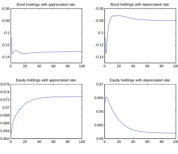
In Table 3, I show the average asset holdings for the three possible outcomes of
experiment 1. The results show that following the adoption of the euro the CEEC will
increase their borrowing and buy domestic equity from foreign investors if the conversion
occurs at the appreciated exchange rate. On the other hand, if there is a depreciation of
the currency at the time of joining the EMU, then one observes debt repayment and a
sale of domestic equity to foreign investors. In this situation, repayment of debt makes
sense as it is denominated in euros, not in the domestic currency. Furthermore, the
permanent depreciation sets in motion a portfolio rebalancing, as in Hau and Rey (2004)
and also found in Marques (2007), in a setting with two large economies. This portfolio
rebalancing means that the representative investor of the CEEC will sell equity on its
tradable sector to foreign investors (who now find CEEC relatively more attractive) and
permanently reduce its claims on future dividends and its future consumption.
Note that the initial asset holdings used for this experiment are indeed very far away
from the bond and equity holdings that one observes in this economy at a stochastic
9
steady state. Given that the CEEC economies are still undergoing a significant economic
transition, I see this as a realistic feature of the model and simulations.
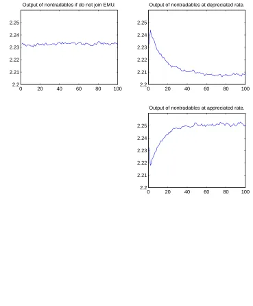
In Figure 1, I show the average path for the trade balance under the various scenarios
of experiment 1. To abstract from the adjustment induced by the fact that the initial
asset holdings are outside the ergodic set, the simulations shown in figures 1 and 2 take as
starting points asset holdings within or close to that set. From the second and third panels
of this figure, it is apparent that the trade balance exhibits the J-curve pattern stated
by Backus et al. (1994). Furthermore, since the consumption of nontradables decreases
following the depreciation (in this case, equivalent to a terms of trade deterioration), as
shown in figure 2, we have that the trade balance improvement that eventually comes
about is countercyclical, an empirical regularity noted by Leonard and Stockman (2002).
Cardi (2007) explains this using habit formation and capital adjustment costs in a small
open economy model where only a bond can be internationally traded.
It is interesting to see that the same behavior can be obtained with less complicated
preferences and fewer restrictions on the menu of internationally traded assets. There
are two mechanisms at play here, one being the slow adjustment of portfolio holdings
due to transaction costs. The other mechanism, that explains the trade balance being
countercyclical is the low degree of substitutability between consumption of tradables and
nontradables. If one assumes constant asset holdings, zero bond holdings, and S = 1, a currency depreciation causes a drop in consumption (and output) of nontradables if
µ >0, which is to say an elasticity of substitution between tradables and nontradables, 1/(1 +µ) of less than one. This way, the gradual improvement in the trade balance caused by the depreciation takes place as output decreases. This result is analogous to
what is found in Cooley and Quadrini (2001) and is detailed at the end of the appendix.
In experiment 2, I compute the average lifetime utility of joining the EMU after
results for this experiment, in Table 4, show that the welfare loss stemming from a 20%
depreciation at the time of entry to the EMU is of 1.65% of lifetime utility. The asset
holdings for the simulation of this experiment are in Figure 4, which shows the expected
pattern of decreased borrowing and equity holdings once the accession to the EMU
hap-pens at the depreciated conversion rate. The magnitude of the portfolio rebalancing is,
nonetheless, small (about 1 percentage point). This is most likely because of the
as-sumption of large transaction costs for equity (in this scenario, almost 2% of aggregate
consumption). By inspection of Figure 3, both the trade balance and the output of
non-tradables behave as expected, with the depreciation causing a protracted improvement
in the trade balance and a decrease in output.
Finally, in experiment 3, I compare the outcomes when joining the EMU at either
conversion rate under certainty or at an uncertain future. The results, in Table 5, show
that joining the EMU with certainty five years from today, with a depreciated currency
(as opposed to joining at the appreciated rate), entails a slightly lower cost to consumers
(of 1.41%) than what can be found under the scenario of uncertain accession date to
the EMU (in this case, 1.98%). However, the average utilities and consumptions under
certainty (regarding date of entry to EMU and conversion rate) are lower than what
is found under uncertainty, at the appreciated conversion rate (under the depreciated
conversion rate, the welfare results are very close).
An explanation for this is the different level of transaction costs implied by the
ad-justment of the asset holdings under the two possible paths (certainty vs. uncertainty).
Specifically, knowing the date and parity for entry in the EMU should set in motion
an immediate portfolio adjustment, whereas with uncertainty the adjustment should be
more gradual. If the initial asset holdings are very far away to what they will be under a
stochastic steady state, the adjustment costs that the investor has to pay are very high
To test this hypothesis, I simulate the economy under certainty and uncertainty
re-garding the timing and conversion rate to the euro for an initial level of asset holdings
very close to the average holdings under the former scenario for the last 50 years of
the sample.10
The results, in Table 6, show that this is a plausible explanation for the
anomaly. In fact, if one removes the impact of the initial portfolio holdings, lifetime
consumption is slightly higher when it is known in advance the timing of joining EMU
and the conversion rate than when this is not known.
5
Conclusions
This paper presents an estimate for the costs for the new member countries of the EU to
adopt the euro as its currency at a depreciated conversion rate. I find that these costs,
in terms of lifetime utility measured in equivalent units of consumption, can be as high
as 1.65% of lost aggregate consumption, for a 20% depreciation. In this scenario, joining
the EMU is portrayed as an uncertain event with a 50% chance of happening within 13.5
years. The cost increases to almost 2% if the median date for EMU entry is only five
years. This value is somewhat lower if the date of entry to the Euro Area is known with
certainty.
The costs of the permanent exchange rate depreciation come from the increased
rel-ative price of imports (trade channel), and the adverse valuation and wealth effects
stemming from the foreign asset positions. Contrary to what is found in Marques (2007)
and in Tille (2005), there is a wealth transfer to foreign creditors because the CEEC hold
only euro denominated foreign debt. On the other hand, since foreign investors want to
keep a constant portfolio share for CEEC equity, there is a clear portfolio rebalancing
effect moving against the consumers in these countries.
10
Finally, the model used in the paper, which assumes transaction costs for both equity
and bonds, and a low elasticity of substitution between tradables and nontradables,
provides an explanation for the J-curve pattern observed for the trade balance and its
countercyclical movement.
An immediate extension to the current work is to have the exogenous interest rate that
the CEEC face on international borrowing to include a pre-EMU accession premium. In
fact, Fagan and Gaspar (2007) argue that a decrease in the interest rates after adopting
the euro was a major contributor to increased consumption in Italy, Spain, Portugal,
and Greece and therefore should be included in welfare calculations for the prospective
EMU members. This is modeled, following Blanchard and Giavazzi (2002), as a drop
in the exogenous interest rate risk premium and does not pose a significant technical
challenge. However, unless there is a tradeoff between the conversion exchange rate and
the increased access to finance for domestic agents, this addition should not matter for
comparative welfare calculations.
One other extension is to consider the effect of fiscal policy. This is a potentially
important extension as fiscal discipline is one of the most stressed (and often most difficult
to comply with) criteria of accession to EMU and, under the Growth and Stability Pact,
remains a permanent constraint after the adoption of the common currency.
Two important and lengthier extensions to this work are to include capital
accumu-lation in the nontradable goods’ sector and production in the traded goods sector. This
can be achieved at the expense of a sizeable expansion of the state space and increase of
the computational burden and for this reason it is left for future work.
A perhaps more challenging extension is to consider the political economy aspects of
currency depreciations and EMU accession. Specifically, considering population
hetero-geneity (be it investor heterohetero-geneity or firm heterohetero-geneity) adds a new and important
in the exchange rate and the terms of trade, others may win. Owners of firms that are
very dependent on export markets or investors that have a low degree of home bias in
their portfolio holdings (and thus own more foreign currency denominated assets) may
benefit and even lobby for weak currency policies and that way influence policy outcomes
at the expense of others. Furthermore, since there are powerful wealth effects in action,
the impact on the distribution of wealth (within a country) of currency movements is
Appendix:
Equilibrium Conditions
Here I present the Euler equations and other equilibrium conditions that can be used to
solve the problem via policy function iteration. I then detail on how the policy functions
are derived. I finally derive the conditions under which, in equilibrium, the consumption
of nontradables declines after a currency depreciation.
1. Equilibrium conditions:
The policy functions for the assets (bond and equity) are given by Chebyshev
poly-nomial fitting over aM×M grid of bond and equity holdings, for each state. Regarding the exchange rate, there are four possible states: join the Euro Zone at the appreciated
exchange rate, join the Euro Zone at the depreciated rate, have a appreciated exchange
rate and not joining the Euro Zone, and have a depreciated exchange rate and not
join-ing the Euro Zone. For each possible state for the exchange rate there are eight possible
combinations for the other exogenous state variables, xt ≡ {Dt, At,Ω∗t} (the shock to
dividends of traded goods, the technology shock in the nontraded goods sector, and the
shock to foreign financial wealth). I call these sets of states 1, 2, 3, and 4, respectively.
After the CEEC adopts the euro, that is, once the economy enters one of the absorbing
states (1 or 2), the equations to be solved, for S ∈ {S,S¯} are:
βEt µ
Qt+1+Dt+1+ 2Qt+1ψ3(θt+2−θt+1)
Qt+ 2ψ3Qt(θt+1−θt)
uT(CT,t+1, CN,t+1, Ht+1)
uT(CT t, CN t, Ht)
PT,t
PT,t+1
= 1, (A-1)
βEt µ
1 +r+ 2ψ2(Bt+2−Bt+1)
1 + 2ψ2(Bt+1−Bt)
uT(CT,t+1, CN,t+1, Ht+1)
uT(CT t, CN t, Ht)
PT,t
PT,t+1
where:
Ht = µ
γA−tµ(
1−λ λ CT t)
1+µ
PT t
¶ρ+1+1µγ
, (A-3)
Qt = a∗
StΩ∗t
1−θt+1
, (A-4)
CT t =
1 PT t
(−StBt+1−Qtθt+1+ (Qt+Dt)θt+St(1 +r)Bt−T Ct), (A-5)
CN t = AtHtγ, (A-6)
PT t = P1t(P2tSt)1−α, (A-7)
and
PN t = µ
1−λ λ
CT t
CN t ¶1+µ
PT t, (A-8)
where the transaction costs, T Ct, are given by (6).
2. Solving for the policy functions:
In the conditions above, the consistency conditions between individual and per capita
aggregate asset holdings already have been imposed, before solving for the policy
func-tions. I can do this because I am only interested in analyzing solutions for this economy
along the equilibrium path.
The solution to this problem yields four policy functions for assets, conditional on the
set of observed prices, Πt≡ {PT,t, PN,t, Qt}: b1(B, θ, x,S¯|Π),b2(B, θ, x, S|Π),f1(B, θ, x,S¯|Π),
of Euler equations (where the expectation operator is taken with respect to xt only): βEt 4 X i=1 µ
(Qt+1+Dt+1+ 2Qt+1ψ3(fi(Bt+1, θt+1)−θt+1))uT(CT,t+1, CN,t+1, Ht+1)
PT,t+1
= (Qt+ 2ψ3Qt(θt+1−θt))(uT(CT t, CN t, Ht)) PT,t , (A-9) βEt 4 X i=1 µ
(1 +r+ 2ψ2(bi(Bt+1, θt+1)−Bt+1))(uT(CT,t+1, CN,t+1, Ht+1))
PT,t+1
= (1 + 2ψ2(Bt+1−Bt))(uT(CT t, CN t, Ht)) PT,t
, (A-10)
together with (A-3)-(A-8). The solutions are then used to build the policy functions for
the non absorbing states (3 and 4): b3(B, θ, x,S¯|Π), b4(B, θ, x, S|Π), f3(B, θ, x,S¯|Π), and f4(B, θ, x, S|Π).
3. Impact of currency depreciation on consumption of nontradables:
From (A-3) and (A-6) one can derive the impact on the output of nontradables of a
change in the exchange rate. This is given by:
∂CN
∂S =a1
µ
(1 +µ)γ 1 +ρ+µγ
∂CT
∂S C
(1+µ)γ
1+ρ+µγ−1
T P
γ
1+ρ+µγ
T +
(1−α)γ 1 +ρ+µγC
(1+µ)γ
1+ρ+µγ
T P
γ
1+ρ+µγ−1
T
, (A-11)
where a1 is an exogenous term and it is implicit the assumption that P1t = P2t = 1.
The output of nontradables decreases following a depreciation if (A-11) is less than zero,
which means:
(1 +µ)∂CT ∂S
1 Ct
+ (1−α)1 S <0
⇔
∂CT
∂S S CT
< 1−α
On the left hand side of (A-12) one has the elasticity of consumption of tradables with
respect to the exchange rate, which is highest in absolute value, the costlier it is to adjust
portfolios. If one assumes that the transaction costs are so high that asset holdings are
constant (making it more likely for (A-12) to be verified), then we can rewrite the above
elasticity as:
∂CT
∂S S CT
=−(1−α)Sα−1−Sα Ct
ψ2B2
<−(1−α)Sα−1 (A-13)
For zero bond holdings and S = 1, (A-12) becomes µ >0. This is to say that for a low degree of substitutability between tradables and nontradables, a depreciation will lower
the output and consumption of the latter. For non zero bond holdings, this remains true
References
[1] Backus, David, Patrick J. Kehoe, and Finn Kydland (1994). “Dynamics of the Trade
Balance and the Terms of Trade: The J-Curve?,” The American Economic Review
84, pp. 84-103.
[2] Blanchard, Olivier, and Francesco Giavazzi (2002). “Current Account Deficits in
the Euro Area: The End of the Feldstein-Horioka Puzzle?” Brookings Papers on
Economic Activity, 2, pp. 147-186.
[3] Bul´ı˘r, Ale˘s, and Kate˘rina ˘Sm´ıdkov´a (2005). “Exchange Rates in the New EU
Aces-sion Countries: What Have We Learned from the Forerunners?” IMF Working Paper
05/27.
[4] Cardi, Olivier (2007). “Another View of the J-Curve,” Macroeconomic Dynamics,
11(2), pp. 153-174.
[5] Cocco, Jo˜ao, Francisco Gomes, and Pascal Maenhout (2005). “Consumption and
Portfolio Choice over the Life Cycle,” Review of Financial Studies, 18(2):491-533.
[6] Cooley, Thomas F., and Vincenzo Quadrini (2001). “The Costs of Losing Monetary
Independence: The Case of Mexico,” Journal of Money, Credit and Banking, Vol.
33, No. 2, Part 2: Global Monetary Integration, pp. 370-397.
[7] ´Egert, Bal´azs, L´aszlo Halpern, and Ronald MacDonald (2005). “Equilibrium
Ex-change Rates in Transition Economies: Taking Stock of the Issues,” The William
Davidson Institute Working Paper No. 793.
[8] Fagan, Gabriel and V´ıtor Gaspar (2007). “Adjusting to the euro,” ECB Working
[9] Greenwood, Jeremy, Zvi Hercowitz, and Gregory W. Huffman (1988). “Investment,
Capacity Utilization, and the Real Business Cycle,”The American Economic Review
June 1988, 78, 402-417.
[10] Hau, Harald, and H´el`ene Rey (2004). “Can Portfolio Rebalancing Explain the
Dy-namics of Equity Returns, Equity Flows, and Exchange Rates?”, American
Eco-nomic Review, 94 (2), pp. 126-133.
[11] Judd, Kenneth L. (1998).Numerical Methods in Economics, Cambridge: MIT Press.
[12] Lane, Philip R., and Gian Maria Milesi-Ferretti (2006). “Capital Flows to Central
and Eastern Europe,” IMF Working Paper 06/188.
[13] Leonard, Greg, and Alan Stockman (2002). “Current Accounts and Exchange Rates:
A New Look at the Evidence,” Review of International Economics, 10(3),
pp.483-496.
[14] Marques, Luis B. (2007) “Welfare Implications of Exchange Rate Changes,”working
paper.
[15] Mendoza, Enrique (2001). “The Benefits of Dollarization When Stabilization Policy
Lacks Credibility and Financial Markets are Imperfect,” Journal of Money, Credit,
and Banking, Vol. 33, No. 2, pp. 440-474.
[16] Mendoza, Enrique G. and Martin Uribe (2000). “Devaluation risk and the
business-cycle implications of exchange-rate management,” Carnegie-Rochester Conference
Series on Public Policy 53, pp. 239-296.
[17] Obstfeld, Maurice, and Kenneth Rogoff (2005). “Global current account imbalances
and exchange rate adjustments,” Brookings Papers on Economic Activity, 1:2005,
[18] Rahn, J¨org (2003). “Bilateral equilibrium exchange rates of EU accession countries
against the euro,” Bank of Finland Institute for Economies in Transition Discussion
Paper No. 11.
[19] Rawdanowicz, Lukasz (2006). “EMU enlargement and the choice of euro conversion
rates,” in M. Dabrowski and J. Rostowski (eds.)The Eastern Enlargement of Europe,
pp. 113-129.
[20] Schadler, Susan, Paulo Drummond, Louis Kuijs, Zuzana Murgasova, and Rachel van
Elkan (2005). “Adopting the Euro in Central Europe: Challenges of the Next Step
in European Integration,” IMF Occasional Paper No. 234.
[21] Schmitt-Groh´e, Stephanie and Mart´ın Uribe (2003). “Closing small open economy
models,” Journal of International Economics 61, pp. 163-185.
[22] Stockman, Alan, and Harris Dellas (1989). “International Portfolio
Nondiversifica-tion and Exchange Rate Variability,” Journal of International Economics, 26, pp.
271-289.
[23] Stokey, Nancy, and Robert E. Lucas (1989). Recursive Methods in Economic
Dy-namics, Cambridge: Harvard University Press.
[24] Swann, Christopher (2002). “Global Investing: Expanding the eurozone may not
contract the currency,” Financial Times, October 24, 2002.
[25] Tille, Cedric (2005). “Financial Integration and the Wealth Effect of Exchange Rate
0 20 40 60 80 100 0.34
0.35 0.36 0.37 0.38
Trade Balance if do not join EMU.
0 20 40 60 80 100 0.345
0.35 0.355 0.36 0.365 0.37 0.375
Trade Balance at depreciated rate.
0 20 40 60 80 100 0.34
0.35 0.36 0.37 0.38
Trade Balance at appreciated rate.
0 20 40 60 80 100 2.2
2.21 2.22 2.23 2.24 2.25
Output of nontradables if do not join EMU.
0 20 40 60 80 100 2.2
2.21 2.22 2.23 2.24 2.25
Output of nontradables at depreciated rate.
0 20 40 60 80 100 2.2
2.21 2.22 2.23 2.24 2.25
[image:31.595.110.479.232.678.2]Output of nontradables at appreciated rate.
0 20 40 60 80 100 2.23
2.24 2.25 2.26 2.27 2.28 2.29 2.3
Output of Nontradables in EMU at appreciated rate.
0 20 40 60 80 100 0.33
0.335 0.34 0.345 0.35 0.355 0.36
Trade Balance in EMU at appreciated rate.
0 20 40 60 80 100 2.23
2.24 2.25 2.26 2.27 2.28 2.29 2.3
Output of Nontradables in EMU at depreciated rate.
0 20 40 60 80 100 0.33
0.335 0.34 0.345 0.35 0.355 0.36
[image:32.595.116.474.226.555.2]Trade Balance in EMU at depreciated rate.
0 20 40 60 80 100 -0.14
-0.12 -0.1 -0.08 -0.06
Bond holdings with appreciated rate.
0 20 40 60 80 100 0.662
0.664 0.666 0.668 0.67 0.672 0.674 0.676
Equity holdings with appreciated rate.
0 20 40 60 80 100 -0.14
-0.12 -0.1 -0.08 -0.06
Bond holdings with depreciated rate.
0 20 40 60 80 100 0.65
0.655 0.66 0.665 0.67
[image:33.595.119.472.230.536.2]Equity holdings with depreciated rate.
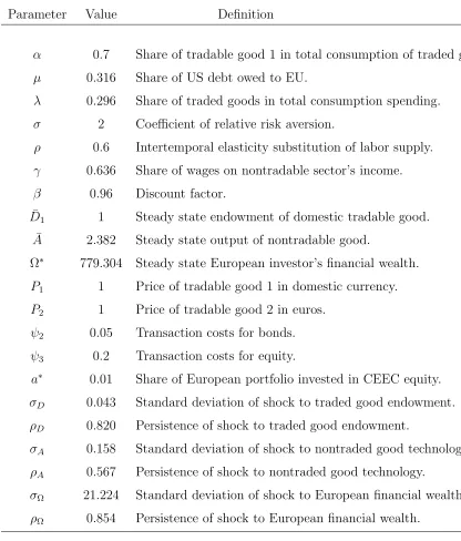
Table 1
Calibration parameters
The table shows the parameter values used to solve the model and perform the numerical simulations.
Parameter Value Definition
α 0.7 Share of tradable good 1 in total consumption of traded goods. µ 0.316 Share of US debt owed to EU.
λ 0.296 Share of traded goods in total consumption spending. σ 2 Coefficient of relative risk aversion.
ρ 0.6 Intertemporal elasticity substitution of labor supply. γ 0.636 Share of wages on nontradable sector’s income. β 0.96 Discount factor.
¯
D1 1 Steady state endowment of domestic tradable good. ¯
A 2.382 Steady state output of nontradable good.
Ω∗ 779.304 Steady state European investor’s financial wealth.
P1 1 Price of tradable good 1 in domestic currency. P2 1 Price of tradable good 2 in euros.
ψ2 0.05 Transaction costs for bonds. ψ3 0.2 Transaction costs for equity.
a∗ 0.01 Share of European portfolio invested in CEEC equity. σD 0.043 Standard deviation of shock to traded good endowment.
ρD 0.820 Persistence of shock to traded good endowment.
σA 0.158 Standard deviation of shock to nontraded good technology.
ρA 0.567 Persistence of shock to nontraded good technology.
Table 2
Welfare results in experiment 1
The first row in the table shows lifetime utility(U), in equivalent units of aggregate consumption, total consumption of traded goods (CT), and total consumption of non traded goods (CN), when the CEEC permanently opt out entering the Euro Zone. The second and third rows of the table show lifetime utility when the CEEC adopt the euro at the current period, at either the normal or the depreciated exchange rate. The last column shows the correlation between the output of nontradables and the trade balance. The initial bond and equity holdings are -1 and 0.8, respectively.
U in % CT in % CN in % rT B,CN
no euro 3.2257 100.00 0.6783 100.00 2.3144 100.00 0.0231 depreciated rate 3.1932 98.99 0.6564 96.77 2.3020 99.46 -0.9924 appreciated rate 3.2550 100.91 0.6974 102.81 2.3245 100.44 -0.9931
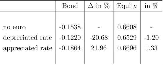
Table 3
Asset holdings in experiment 1
The first row in the table shows average bond and equity holdings, when the CEEC permanently opt out entering the Euro Zone. The second and third rows of the table show bond and equity holdings when the CEEC adopt the euro at the current period, at either the normal or the depreciated exchange rate. Percent variations in bond holdings mean increases in borrowing.
Bond ∆ in % Equity in %
[image:35.595.160.436.566.677.2]Table 4
Welfare results in experiment 2
The first row in the table shows lifetime utility(U), total consumption of traded goods (CT), and total consumption of non traded goods (CN), when the CEEC adopt the euro in an uncertain future at the normal exchange rate, with a median waiting period of 13.5 years. The second rows in the table shows lifetime utility when the CEEC joins the Euro Zone at the deppreciated conversion rate. The initial bond and equity holdings are -1 and 0.8, respectively.
U in % CT in % CN in %
uncertain date depreciated rate 3.2145 98.35 0.6699 94.39 2.3248 99.00 uncertain date appreciated rate 3.2685 100.00 0.7097 100.00 2.3482 100.00
Table 5
Welfare results in experiment 3 (version 1).
The first row in the table shows lifetime utility(U), total consumption of traded goods (CT), and total consumption of non traded goods (CN), when the CEEC adopt the euro in an uncertain future, at either the normal or the depreciated exchange rate, with a median waiting period of 5 years. The second and third rows in the table show lifetime utility when the CEEC join the Euro Zone after 5 years with certainty, at either conversion rate. The initial bond and equity holdings are -1 and 0.8, respectively.
U in % CT in % CN in %
uncertain date at depreciated rate 3.2097 98.02 0.6678 93.95 2.3251 98.94 uncertain date at appreciated rate 3.2747 100.00 0.7108 100.00 2.3500 100.00
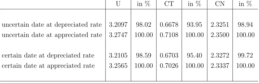
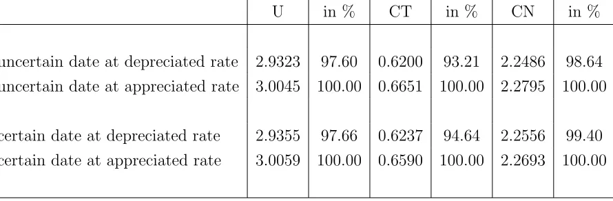
[image:36.595.75.528.561.706.2]Table 6
Welfare results in experiment 3 (version 2).
The first row in the table shows lifetime utility(U), total consumption of traded goods (CT), and total consumption of non traded goods (CN), when the CEEC adopt the euro in an uncertain future, at either the normal or the depreciated exchange rate, with a median waiting period of 5 years. The second and third rows in the table show lifetime utility when the CEEC join the Euro Zone after 5 years with certainty, at either conversion rate. The initial bond and equity holdings are -0.1803 and 0.6666, respectively.
U in % CT in % CN in %
uncertain date at depreciated rate 2.9323 97.60 0.6200 93.21 2.2486 98.64 uncertain date at appreciated rate 3.0045 100.00 0.6651 100.00 2.2795 100.00