On Stable Plane Vortex Flows of an Ideal Fluid

On Stable Plane Vortex Flows of an Ideal Fluid

O.V. Troshkin

Institute for Computer Aided Design, Russian Academy of Sciences, Moscow Physical-Technical Institute, Russia

Copyright©2016 by authors, all rights reserved. Authors agree that this article remains permanently open access under the terms of the Creative Commons Attribution License 4.0 International License

Abstract

2D-flows of an ideal incompressible fluid are treated in a rectangular. If analytical (resolved in series of powers of coordinates), the stationary flows are uniquely determined with the inflow vorticity. When excluded vortices of a spectral origin, such flows prove to be stable.

Keywords

Ideal Incompressible Fluid, 2D-flows, Impenetrable or Periodical Walls, Analytical Stationary Vortices, Nonlinear Stability

1. Vorticies of 1883 and 1941

Apparently, the idea of hydrodynamic stability was born in 1883 from “particular cause” of O. Reynolds [1] and “disturbed equilibrium” of J.W.S. Rayleigh [2] to give rise soon to velocity pulsations and correlations of W. Thomson [3] referred now to as turbulent stresses. The phenomenon involved had initially been found closely related to circulations as vortices spontaneously originated in a fluid motion. However, some of them continue stubbornly to reveal their non–linear stability (by A.M. Lyapunov [4]), as follows.

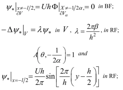
Counter–flow circulations. In 1941, P.A.M. Dirac as a participant of the first atomic project (Tube Alloys) had unexpectedly developed an artificial idea (of a chemical origin from R.S. Mulliken [5] and H.C. Urey [6]) on mass separation in the uranium hexafluoride. In the almost invisible rotating gas rarefied to centre and adhering to the boundary of the rotor (cylinder) of the future industrial centrifuge, he had seen [7] a natural cause required for the desired fractionating of the isotope mixture (consisting basically of U–235 and U–238 [8]). The cause proved to be the counter–flow circulation [9] in the form of a vortex ring [10–12] twisted round the axis as shown in the Fig. 1.

[image:1.595.336.509.240.451.2]

The rotation of an air mass (mesocyclone) in the atmospheric swirl (tornado) is accompanied with the same circulation (see Fig. 1). It could hastily be taken for a secondary flow originating in a rotating medium owing to the loss of stability as with Taylor vortices taken to be the counter–flows of the Couette flow between cylinders that arise inevitably as` bifurcations [13–15] due to the Reynolds number [1].

Figure 1. The counter–flow vortex as a small tornado in the rotating rotor of the gas centrifuge.

Meanwhile, the absence of the internal rigid wall (in the form of the cylinder) in a region around air swirl or hexafluoride gas center (of which the first one has always the pressure drop [16, § 1] while the second turns out to be a rarefied gas [8, 9, 17]) seems to play a crucial part in the forming of their true flow pattern that is reduced not to a secondary velocity field (as with Taylor vortices) and proved to be a basic (non–disturbed) flux (as with the Couette flow). As we shall see below, a plane vortex in a channel delivers such an example of a basic (or undisturbed) flow related directly to the counter–flow circulation.

Rip–flow vortices. In the same year (1941), G. I. Taylor had exactly estimated parameters of what that had been subsequently declassified [18] and realized in the atomic mushroom [19]. For small scales, it had evidenced on the non–linear stadium of RTI, or the hydrodynamic instability come from the first (linear) considerations of Rayleigh [2] and Taylor [20] validated first by D.J. Lewis [21].

[image:2.595.73.545.79.161.2]

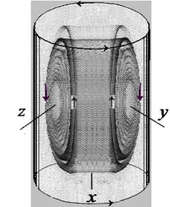
Figure 2. Rip–flow mushrooms originating since 40

µ

s

(microseconds) behind the shock front crossing normally the disturbed boundary from Argon to Xenon in RMI [23,24].

Meanwhile, the discontinuity of the normal velocity component in the contact boundary seems to be a not less significant cause for RM–type instabilities then the difference in densities of two media contacted: familiar sea water waves striking a board of a ship in a calm harbor produce similar vortex mushrooms originating (after impact) and resembling that usually produced with breakers crossing sand bars off the shore when the water has to travel back out to sea through a gap in the sand bar, creating a fast (and dangerous) rip current.

2. Flow Patterns

Following W. Wolibner [26], V. I. Yudovich [27] and T. Kato [28], we shall consider the initial value problem

( )

0 0 0

,

_t

,

,

u

u

₌

=

u

u

x y

,

(

x y V V

,

)

∈ =

_lh, or

2

x l

≤

,

0

≤ ≤

y h

,

posed for such smooth (infinitely differentiable everywhere in

V

for t≥0) horizontal and vertical velocity components u u t x y=

₍

_{, ,}

₎

and u of a plane non–stationary

flow

u

,

u

(of an ideal incompressible fluid in a rectangular

V

) that form a specific (divided by a constant density) pressure _{p p t x y}=

₍

_{, ,}

₎

[10], or satisfy the 2D–system of Euler hydrodynamical equations:

(1)

Components

u

,

u

are taken to be disturbances (with

deviations

u u

−

_∗,

u u

−

_∗) of a smooth stationary flow with components

(

,

)

u u x y

=

∗ and

u u

=

∗

(

x y

,

)

for

∂ ≡

t

0

. (2)

a pressure

p p x y

=

∗

(

_,

)

in (1).

The flow

u

,

u

is to satisfy the following boundary conditions (PF), (BF) or (RF) with the vorticity

x

u

y

ω u

=

−

(3)

prescribed in inflow parts of the boundary

∂ =

V V V

\

(and in accordance with initial data).

The pass–flow

2

x l

u

_=

=

U

,

u

_y=0,h

=

0

,

ω

_{x l=− 2}

= Ω

,

,

U

Ω =

const

,

U

>

0

,

t

≥

0

, PF

where the aspect ratio

α

>

0

and the vorticity factor

β

−∞ < < ∞

,

h l

α

=

and

β

= Ω

h U

(4) originate with critical points

±

β

₀,

( )

0 0

0

β

=

β α

>

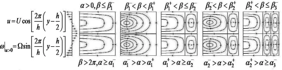
in PF, (5) of bifurcations in the Fig. 3.

Figure 3. Pass–flow patterns with bifurcations at critical points ±β α₀

_{( )}

.

The bay–flow

2

2

x l

Uy

u

U

h

=−

= −

,

u

x l= 2

=

0

,

u

y=0,h

=

0

,

2, 0 x l u

ω

=−

>

= Ω

, t≥0, (BF)

inheriting parameters (3) with another critical points,

( )

0

[image:3.595.62.299.76.329.2]

Figure 4. Bay–flow patterns with critical points

β α

_±

( )

.

The rip–flow

(RF)

(the periodicity is assumed to be valid for all the derivatives) and parameters (4) including critical points

(

₂

₁

)

2 2

2

8

m

m

πα

β

−

₌

−

₊

π

_,

_α

_>

₀

_,

1,2,...

m

=

in RF, (7) and excluding some of spectral points

2 2

0

2

m m

m

πα

β

+

₌

β

₌

_,

_α

_>

₀

_{, (8)}

or points of spectral reconstructions depicted in the Fig. 5 with disappearing of positively, i.e. right–hand (or negatively, i.e. left–hand) oriented vortices (like in PF and BF) at the left side of rectangular

V

and originating of negatively (positively) oriented spectral circulations at the right side (respectively) when the parameter

_λ

₌

₂

_πβ

_h

2 _jumps

over the eigenvalue

λ

_m,1 from (9).

Each of the treated problems (with the inflow vorticity prescribed) have the unique non-stationary smooth solution (for any values of parameters involved) by Yuodivich theorem [27]. Existence and uniqueness of the corresponding stationary solution exclusively in the class of analytical functions are proved in [12, 16, 29, 44].

The paper is aimed to study the stability of PF-, BF- and RF-flows for different values of parameters (4). Such a study is possible for the known non–stationary inflow vorticity theorem (of existence and uniqueness) [27] saying that for any smooth initial data

u

_{0 0}

,

u

_∈

C V

∞

( )

_{(real–valued}

functions infinitely differentiable at every point of the closure

V

of the region

V

), the corresponding initial PF–, BF– or RF–problem (1) has the unique smooth non–stationary Euler flow

u

,

u

(with smooth velocity components

u

,

u

) from the corresponding non–stationary class _{C t}∞

(

_≥0,V

)

_{that satisfies initial conditions and}

equations (1) for a smooth pressure

p

and any values (4).

Figure 5. Rip–flow patterns with bifurcations at critical points β β₁−_{, 2}−_,...(or

1, ,...2

α α− − _{) and reconstructions at spectral points}

1, ,...2

β β+ + _(or

1, ,...2

[image:3.595.69.545.468.586.2]

The another known restriction in the classical stability [4] is the necessary uniqueness of the corresponding stationary flow

u

_∗

,

u

_∗. According to the so called stationary inflow (or outflow) vorticity theorem from[12, § 5], [16, § 7] or [29, § 1], for any problems PF, BF or RF there is a unique stationary smooth Euler flow

u

_∗

,

u

_∗ (for a pressure

p

_∗) provided that two following conditions (i) and (ii) are fulfilled:

(i) velocity components

u

_∗ and

u

_∗ are to be analytical, or of the class

_{C C V}

∗

₌

∗

( )

_⊂

_C

∞_{, i.e. approximated with}

polynomials of any order, or decomposed in series of powers

(

x x− 0

) (

m y y− 0

)

n,

m n

,

=

0,1,2,...

, convergent near every point

x y V

₀

,

₀

∈

;

(ii) parameters (4) have to except of spectral points

( )

n n

m m

β

=

β α

as corresponding to ordered eigenvalues

2 2

2

2

n

2

n m

m

πβ

_h

π

_l

m

π

_h

n

λ

=

=



_

 

_{ }

+



_



 



,

2 2 2

2 0

1

2

2

2

n

m

m

πα

n

πα

β

=

+

π

≥

β

=

, in RF,

{ }

λ

_mn

=

{ } {

λ

_k

=

...

>

λ

₂

>

λ

₁

}

,

2 0

1 1

π

_l

λ

=

λ

_{=  }

 

 

,

, ,

1 1,2,...

k m n

+ =

, (9) with corresponding eigenfunctions

ϕ

_mn

( )

x y

,

as satisfying

n n n

m m m

ϕ

λ ϕ

−∆

=

in

V

,

2

0

n m x l

ϕ

=

=

, 0

0

y h n m y

ϕ

=

=

=

in

RF,

or 0

(

_,

)

( )

_sin

2

m

x y

S x

m

l

x

m

_l

π

ϕ

=

=



_



_

−



_



_









for

n

=

0

,

(

,

)

( )

sin

2

,

( )

cos

2

n

m

x y

S x

m

π

_h

ny

S x

m

π

_h

ny

ϕ

=

for

n

>

0

,

{ }

ϕ

_mn

=

{ }

ϕ

_k

=

{

..., ,

ϕ ϕ

_{2 1}

}

. (10) Conditions (i) and (ii) are used below.

3. Zonal Potentials

As is well known, for a pair of smooth real-valued functions _{q q}x_, y_{∈C t}∞

₍

_≥0,V

₎

_{given in a one-connected}

region like a rectangular

V

, the absence of the vorticity 0

y x

x y

q − =q in V (for

t

>

0

), assumes their gradientness,

or the existence of the classical potential _{p C t∈} ∞

₍

_>0,V

₎

such that x x

q = −p and y y

q = −p in

V

[30]. For a

rectangular with periodical walls

y

=

0,

h

(forming a topological cylinder, or a ring on a plane with the Euclidian metric) we have the following

Lemma 1. Smoothness _{q q}x_, y_{∈C t}∞

(

_≥0,V

)

_{and condition}

0

y x

x y

q

− =

q

,

( )

x y V

,

∈

with periodicity

,

0

0

y h x y

y

q

=

=

=

, t≥0

(including all the derivatives) imply the gradientness

x

x

q

= −

p

and

q

y

= −

p

_y,

( )

x y V

,

∈

,

for a zonal potential of the form

(

)

(

)

(

)

(

)

(

)

2 0

, ,

, 2,

1

l h y

_{, ,}

_{, ,}

x

p t x y

p t l

h

q t

y dy d

p t x y

h

x

x

=

+

′

+

_∫

_∫

+

,

(

, ,

)

_yh y

(

, ,

)

1

₀h h

(

_y y

(

, ,

)

)

p t x y

q t x

d

q t x

d dy

h

h h

h h

′

=

_∫

−

_{∫ ∫}

,

( )

x y V

,

∈

, Proof. Really, we have

which states the required gradientness.

The cited formula for

p

follows from a general criterion of gradientness and abc-theorem [31-33] (complementing alternatively the classical orthogonal decompositions of H. Weyl [34] and O.A. Ladyzhenskaya [35]).

(11)

Then the function y relates to the vorticity (3) with the Helmholtz vorticity equation [36]:

0

t y x x y

ω y ω y ω

+

−

=

,

−∆ =

y ω

in

V

for

0

t

>

and

∆ = ∂ + ∂

2_x 2_y, (12) and boundary conditions

V

Uy

y

_∂

=

in PF, _2,

0x ly h

1

y

Uy

h

y

=− < <





=

_

−

_





,

2,

0

x l V

y

≠−

∂

=

in BF,

2

2

sin

2

2

x l

Uh

_h

y

h

π

y

π

=−









=

_

_

−

_

_









,

y

x l= 2

=

0

,

0

0

y h y

y

=₌

=

in RF,

and _2,

0 x l u

ω

=−

>

= Ω

in PF, BF,

2, 0

2

sin

2

x l u

h

y

h

π

ω

=−

>









= Ω

_

_

−

_

_









in RF, (13)

or

( )

2, ₀

0 x l u

ω

=−

µ y

>

=

,

with ₀

( )

, PF, BF,

, RF,

in

s

s in

µ

λ

Ω



= 



2

2

2

Uh

h

π

πβ

λ

=

Ω

=

,

−∞ < < ∞

s

(14)

Namely,

Statement 1. In the class

C

∞

₌

C t

∞

(

_≥

0,

V

)

_{, problems} (1), (PF), (BF) and (RF) for functions

u p

, ,

u

, are equivalent to problems (12)-(14) for functions

y ω

,

.

Proof. The equivalence noted follows from lemma 1 and

Gromeka–Lamb identities

and

2 2

2

x y

y

u

u

u

+

uu

=



_

+

u



_

+

u

ω





so

(

) (

)

( ) ( )

x y _x x y _y

y x x y

x y

u

uu

u

u

u

uu

u

ω

uω

y ω y ω

+

−

+

=

=

+

=

−

and

q

_xy

− =

q

x_y

ω y ω y ω

_t

+

_{y x}

−

_{x y} for

q

x

= +

u uu

_{t x}

+

u

u

_y and

y

t x y

q

= +

u

u

u

+

uu

, which completes the proof.

4. Spaces with a Volume

In terms of Lie groups the vortex equation in (12) describes rotations

y

(i.e. angular velocities) of an ideal

(without friction) top (a rigid body with a fixed point) with

inertia

A

= ∆

(corresponding to the matrix of inertia of the ordinary top) which kinetic momentum is

A

y ω

=

(the vorticity), so the equation (12) proves to be the momentum equilibrium condition in the linear space tangent to the group

( )

SDiff V of diffeomorphisms _{V →V}t _{of the flow region}

V

conservating the deforming element of volume

t

dV dV

=

(the third equality in (1)) [37]:

0

t

A

y y

+ ×

A

y

=

,

A

y

= −∆ =

y ω

, where

y x x y

y ω y ω y ω

× =

−

(15) the Poison’s brackets.

On the other hand, following [38], instead of Lie groups we shall treat the vortex equation (12) (or (15)) in terms of Lie algebras (the latter are generally being introduced independently of the former). To be more precisely, we shall consider (15) in the set

M

of smooth (infinitely differentiable) real-valued functions

ϕ ϕ

=

( )

x y

,

in the closure

V

of the region

{

2,0

}

h l

V V

=

=

x l

<

< <

y h

.

( )

M C V

=

∞ in PF, BF and

( )

{

:

0

0

}

y h y

M

ϕ

C V

∞

ϕ

=

=

=

∈

=

in RF, supplied with a metric (a scalar product) and a normal (a vector product, or a commutator),

2 2 0

l h

l

dxdy

ϕ y

₋

ϕy

− ∞ < ⋅ =

_∫

_∫

< ∞

and

ϕ y ϕ y

× =

_{y x}

−

ϕ y

_{x y}

∈

M

for

ϕ y

,

∈

M

, (16) respectively. Then the set

M

proves to be a quasi-compact algebra, or a linear space with a volume

ϕ y χ

⋅ ×

(a tree-linear form) invariant to cyclic permutations

ϕ y χ y χ ϕ

⋅ × = ⋅ ×

for

y χ

,

∈

M

and

1

M

ϕ

∈

where

M

₁

=

{

ϕ

∈

M

:

ϕ

_∂V

=

0

}

in PF,

BF and (17)

in a linear subspace

M

₁

⊂

M

which is dense sub-set in

M

(with respect to the metric) and a sub-algebra of

M

(with respect to the normal) [16, 38].

5. Stationary Solutions

Let us construct stationary flows in Fig. 3-5. For them, the vorticity

( )

x y

,

0

( )

y

_∗

ω

_∗

µ y

_∗

−∆

=

=

in

V

with (13) (18)

is given by (14). For flows in Fig. 3, 4 it is constant and the corresponding flows are determined by two following functions:

Lemma 2. Analytical functions

(

)

,

,

X Y

,

Φ Γ = Φ Γ

,

X

≤

1 2

α

,

0

≤ ≤

Y

1

, or

(

)

1

1

,

X Y

∈ =

V V

α α , satisfying equations

0

XX YY

Φ + Φ =

and

−Γ − Γ =

_{XX YY}

1

in

{

}

1

1

1 2 , 0

1

V V

_α

=

_α

=

X

<

α

< <

Y

, and boundary conditions

(

)

1 2

1

X=− α

Y

Y

Φ

=

−

and

0,1 1 2 V

0

Y= X= α ∂ α

Φ

= Φ

= Γ

=

on

∂ =

V V V

_{α α}

\

_α , are symmetric

(

X Y

,

)

(

X

,1

Y

)

Φ

= Φ

−

,

(

X Y

,

)

(

X Y

,

)

(

X

,1

Y

)

Γ −

= Γ

= Γ

−

in

V

_α,

and convex–concave,

0

XX

Φ >

,

Φ <

_YY

₀

,

Γ

_XX

<

₀

,

Γ <

_YY

0

in

V

_α , with normal derivatives

( )

0

_{0,0 0}

Y Y

Γ =Γ

>

,

Φ = Φ

_{X X}

(



1 2 ,1 2

α

)

<

0

and

0

X X

− +

Γ = −Γ >

.

Proof. The analyticity and the symmetry of Φ and Γ are provided by the classical formulae [39, 40]. Convex–concave properties noted follow from maximum principle, lemma on normal derivative [41] and some extended versions [12, 16] of topological constructions of M. Morse and M. Heins [42, 43] completing the proof.

Statement 2. Each of the PF-, BF-, RF-problems in (13), (14), (18) possesses an analytical solution

y y

=

_∗ with

(

)

(

,

)

Uh Y

X Y

y

_∗

=

+ Γ

β

in PF,

(

)

(

)

(

,

,

)

Uh

X Y

X Y

y

_∗

=

Φ

+ Γ

β

in BF ,

where

X x h

=

and

Y y h

=

for

−∞ < < ∞

β

(19) and

(

,

)

sin 2

1

2

2

Uh A X

Y

y

θ

π

π

∗

=









−

















in RF

where

2

₁

2

π

β

θ

α

π

=

−

,

(

,

)

sh 1 2

(

)

,1 2 ,sin 1 2

(

)

sh sin

X X

A Xθ α θ αX α θ

θ θ

− −

   

   

= −

for

_β

_<

₂

_π

,

_β

₌

₂

_π

,

_β

_>

₂

_π

and 0

m m

β β

_≠

+

₌

β

₍

_{θ π}

_≠

_m

_),

_m

₌

_1,2,...

_{, (20)}

for any

β

in (PF), (BF) and for

β β

≠

_mn ,

,

1 1,2,...

m n

+ =

in (RF), respectively. Proof. Really, we have:

(

)

2 XX YY

V V

Uh

h

α

β

y

_∗

− ∆

= −

Γ

+ Γ

= Ω

, in PF, BF,

V

UhY Uy

y

_{∗ ∂}

=

=

in PF;

2 1 2

1

x l

Uh

X α

Uy

_h

y

y

_{∗ =−}

=

Φ

₌₋

=



_

−



_

1 2 ,

2, X

0

x l

V

V

Uh

α

α

y

_∗ ≠− ≠−

∂

∂

=

Φ

=

in BF;

V

y

_∗

λy

_∗

− ∆

=

in

V

,

2

2

h

πβ

λ

=

, in RF;

1

,

1

2

A

θ

α



₋



₌









and

2

₂

sin

2

₂

x l

Uh

_h

y

h

π

y

π

∗ =−

=

_





_





−

_









_

in RF;

which completes the proof.

Statement 3. Critical and spectral points as corresponding to topological bifurcations in Fig. 3-5 and spectral reconstructions in Fig. 5 are

( )

0

0

1

Y

0

β α

= Γ >

in PF,

( )

_{X X X X}

0

β α

+ − + +

−

= Φ

Γ = −Φ

Γ <

,

( )

_{X X}

0

β α

− −

+

= −Φ

Γ >

in BF

β

m− (or

α

m− ) from (7)

and

m

β

+

(or

α

_m+ ) from (8),

m

=

1,2,...

, in RF, (21) respectively. Bifurcations take place when varying parameters (5) abandon zones free of vortices

0 0

β β β

−

≤ ≤

inPF,

β

₋

≤ ≤

β β

₊ inBF,

( )

1

β β α

_≤

− _,

_α

_>

₀

_{, inRF (22)}

where the maximum principle is valid (or where

(

y y

_{∗ ±}

)

0

±

−

≤

everywhere in

V

) and fall into vortex zones where

0

β

< −

β

or

β β

>

₀ inPF,

β β

<

₋ or

β β

>

₊ inBF,

1 1

β

−

_{< <}

β β

+

,

α

>

0

(or ₁

α α α

−

> >

₁+,

β

>

2

π

)

inRF,

(

)

2 2

1 2 1

2

8

m

m

β

−

₌

₋

πα

₊

π

_,

2 2

0

2

m m

m

πα

β

+

₌

β

₌

_,

_m

₌

_1,2,...

_{, (23)}

where the maximum principle is violated (or

(

y y

_{∗ ±}

)

0

±

−

>

somewhere in

V

). Spectral circulations in RF come when increasing (when diminishing) the parameter

β

(or the parameter

α

) jumps over the first

spectral point

β

₁+ _{(over the point 1}

α

+) and falls into zone of spectral circulations zone

0

1 1 mn

β β

_>

+

₌

β

_≥

β

_, n

m

[image:7.595.79.282.74.222.2]

β β

≠

,

m n

,

+ =

1 1,2,...

(24) Bifurcations and reconstructions are repeated as shown in Fig. 5.

Proof. Really, we have in (20)

( )

0

(

)

( )

0

0,0

0

y

U

Y

y

_∗

= Γ

β β

+

≥ <

for

β

≥ < −

( )

β

₀

and

( )

0

(

)

( )

0

0,

0

y

h U

Y

y

_∗

= Γ

β β

−

≥ <

for

β

≤ >

( )

β

₀ in PF,

(

2, 2

)

(

) ( )

0

x

l

h

U

X

y

−

β β

∗

−

= Γ

−

+

≤ >

for

( )

β

≤ >

β

₊ and

(

2, 2

)

(

) ( )

0

x

l h

U

X

y

−

β

β

∗

= Γ

−

−

≤ >

for

( )

β

≥ <

β

₋ in BF,

which assumes the patterns changes as depicted in Fig. 3, 4. As to RF-flows in Fig. 5 follows immediately from formulae (20). Necessary details are discussed in [12, 16].

Theorem1. For any aspect ratio

α

>

0

and vorticity factor

−∞ < < ∞

β

in PF, RF, RF except of spectral points (8) in RF, the problem (12)-(14) has a unique analytical stationary solution

y ω

_∗

,

_∗ determined by (18)-(20).

Proof. Really, as being valid near a boundary point for any computed functions

y

_∗

( )

x y

,

and

ω

_∗

(

x y

,

)

,

( )

x y V

,

∈

, the relation

ω

_∗

=

µ y

₀

( )

_∗ with a given computed dependence

µ

₀

( )

s

,

−∞ < < ∞

s

, as in (17), is valid everywhere in

V

due to the uniqueness of analytical continuation [12,16, 30].

6. Pass– and Bay–flow Stability

Following [38, 44-47], we shall consider now the stability of the computed PF–, BF–, RF-flows as stationary points (or

equilibrium positions)

y ω

_∗

,

_∗ of the top from section 3 in

M C

₌

∞_{. Substituting sums}

y y

=

_∗

+

ϕ

and

ω ω ζ

=

_∗

+

into (12) (or (15)) and (13) and taking into account that

0

t

ω

_∗

=

,

y ω

_∗

×

_∗

=

0

,

ω

_∗

=

A

y

_∗, we come to the equation in variations

0

t

( )

x y V

,

∈

, (25) for deviations

ϕ ζ

,

of

y ω

,

from

y ω

_∗

,

_∗ in

C

∞ satisfying homogeneous boundary conditions

0

V

ϕ

_∂

=

in PF, BF,

ϕ

_{x l= 2}

=

₀

,

ϕ

y h_y=₌₀

=

0

in RF, or

1

M

C

ϕ

_∈

₌

_

∞

2,

0

0

x l u

ζ

∗

=−

>

=

in PF, BF, RF, 0 0

0

y h y h

y y

ϕ

=₌

=

ζ

=₌

=

in RF,

y

u

_∗

=

y

_∗ . (26) Multiplying (25) scalar by

ζ

and using the quasi-compactness (17),

0

ζ ϕ ζ ϕ ζ ζ

⋅ × = ⋅ × =

(

ζ ζ

× =

0

) and

ζ ϕ ω

⋅ ×

_∗

= ⋅

ϕ ω ζ

_∗

×

,

for

ϕ

∈

M

₁ and

ω ζ

_∗

,

∈

M

, together with the familiar equality

(

)

2

ζ ζ

⋅ =

_t

ζ ζ

⋅

_t, we obtain the energy momentum identity

,(27)

with relaxation

ζ y ζ

⋅

_∗

×

and generation

ϕ ω ζ

⋅

_∗

×

.

Statement 4. For the inflow vorticity prescribed the relaxation is non-negative:

0

ζ y ζ

⋅

∗

× ≥

.

Proof. Really, we have

( ) ( )

2 2

1

2

y x x y

x y

u

ζ y ζ y ζζ y ζζ

ζ

u ζ

∗ ∗ ∗

∗ ∗

⋅

× =

−

=





=

_

+

_





,

y

u

_∗

=

y

_∗ ,

u

_∗

= −

y

_∗x, so

2 2

2 0

2

2 2

0 2

2 0

2

0

h x l

x l

l y h h

y x l

l

u

dy

dx

u

dy

ζ y

ζ

ζ

u ζ

ζ

=

∗ ∗ ₌₋

=

∗ ₌ ∗ ₌

−

⋅

× =

_∫

+

+

_∫

=

_∫

≥

,

(since

2

0

x l

ζ

₌₋

=

, 2

0

0

y h y

u ζ

∗ =₌

=

and

u

_{∗ =x l 2}

≥

0

)

which completes the proof.

Theorem 2. For any aspect ratio and vorticity factor in (4), PF- and BF-flows are stable (non-linearly).

Proof. Really, in this case the generation is vanishes

0

ϕ ω ζ

⋅

_∗

× =

(

ω

_∗

=

const

), so the statement 4 implies in (27) that

(

ζ ζ

⋅

)

_t

≤

0

, hence, 2 2 0

ζ

≤

ζ

in PF, BF, t≥0 (

ζ

₀

=

ζ

_t=0).

7. Rip-flow Stability

Further, multiplying (25) scalar by

ϕ

and using the quasi-compactness (17),

0

ϕ ϕ ω

⋅ ×

_∗

= ⋅ × =

ϕ ϕ ζ

,

ϕ

∈

M

₁,

,

M

ω ζ

_∗

∈

, together with equalities

(

)

(

)

1

1

2

2

t t _{t t}

ϕ ζ

⋅ = − ⋅ ∆ =

ϕ ϕ

∇ ⋅∇

ϕ ϕ

=

ϕ ζ

⋅

(

ζ

= −∆

ϕ

), we take the familiar energy identity

(

)

1

₀

2

ζ ϕ

⋅

t

+ ⋅

ϕ y ζ

∗

× =

. (28)

The statement 4 and (27) imply the energy momentum inequality

(

)

1

₀

2

ζ ζ

⋅

t

+ ⋅

ϕ ω ζ

∗

× ≤

. (29)

Multiplying (28) by

λ

and substituting from (29) we come to the energy defect inequality:

(

)

(

)

1

₀

2

ζ ζ λϕ

⋅ −

t

+ ⋅

ϕ ω λy

∗

−

∗

× ≤

ζ

. (30)

As in [38], for rip-flows, we introduce the scalar square

:

:

B M

→

M

h

→

B

h

of inertia

:

:

A M

→

M

x

→

A

x

, or the dissipation to be determined in the more narrow set then the latter,

A A

h y h y

⋅

= ⋅

B

,

h

∈ ⊂

D M

₁

⊂

M

,

{

1

:

x x l ₂

0

}

D

=

M

h

₌

=

,

generally non-commutative with inertia,

A

= −∆

and

B

= ∆∆

(that can be verified immediately). According to [44, statement 4] we have Lemma 3. The least principal eigenvalue

1

1 1

1 _{, 0}

1 1

inf

M

A

A

x x

x x x

x

λ

x x

x x

∈ ≠

⋅

⋅

=

=

⋅

⋅

,

1 1 1

A

x

=

λ x

,

x

₁

∈

M

₁

(

x

₁

≠

0

),

no more than the least joint eigenvalue

1 1

1 _{, 0}

1 1

inf

D

A A

A

A

A

A

h h

h h

h

h

µ

h h

h

h

∈ ≠

⋅

⋅

=

=

⋅

⋅

,

1 1 1

B

h

=

µ h

A

,

h

₁

∈

D

(

h

₁

≠

0

).

Proof. Really, the Cauchy–Bunyakovsky inequality,

1 1 1 1 1 1

1 1

1 1 1 1 1 1

A

A

A

A

A

h

h

h

h x

x

µ

λ

h

h

h h

x x

⋅

⋅

⋅

=

≥

≥

=

⋅

⋅

⋅

,

proves the lemma.

Remark 1. The same is true as to subsequent ordered principal and joint eigenvalues:

λ

_k

≤

µ

_k for

1

k k

λ

<

λ

₊ and

µ

_k

<

µ

_k+1,

k

=

1,2,...

.

The fact that

D

is dense in

M

₁ [40] with respect to the norm

2 2 2

x y

ϕ

ϕ

ϕ ϕ

ϕ

ϕ ϕ ϕ ζ

∇

= ∇ ⋅∇ =

+

= − ∆ = ⋅

,

ζ

= −∆

ϕ

,

ϕ

∈

M

₁, implies

(31)

As a consequence,

Theorem 3. For given inflow vorticity

Ω >

0

and sufficiently long period

2

h l

β

π

>

, or

2 0 1

πα

₂

β β

<

=

, or

λ λ

<

₁,

2

2

h

πβ

λ

=

,

(32)

the RF-flow is stable:

0 2

₂

h

ϕ

ϕ

π α

β π

∆

∇ ≤

−

,

t

≥

0

(

ϕ

₀

=

ϕ

_t=0).

Proof. Really, we have

ω

_∗

=

λy

_∗

in (30). So

(

)

(

ζ ζ λϕ

⋅

−

)

_t

≤

0

,

t

>

0

, and (31) implies

The poof is complete.

Let us note that despite of the same aspect ratio

h l

α

=

and analogous inequality α α> ₀, the stability condition (32) for the rip-flow in Fig. 5 proves to be in opposition to that used in the case of classical channel, with the

l

as a period (in addition to or instead of the only period

h

in our case), and for Kolmogorov and Reynolds sinus-profiles as stable with

α

₀

=

1

and some

0

0.592<

α

<0.593, respectively [44-47].

This work was supported by Russian Science Foundation, project no. 141100719.

REFERENCES

[1] Reynolds O. An experimental investigation of the circumstances which determine whether the motion of water shall be direct or sinuous, and of the law of resistance in parallel channels // Phil. Trans. R. Soc. Lond. 1883. V.174. P. 935–982.

[2] Rayleigh S. J. W. Investigation of the character of the equilibrium of an incompressible heavy fluid of variable density // Proceedings of the London mathematical society. 1883. V.14 , P. 170–177.

[3] Thomson W. On the propagation of laminar motion through a turbulently moving inviscid liquid // Phil. Mag.1887. Ser.5.V.24.Iss.149. P.342–353.

[4] Lyapunov A.M. The General Problem of the Stability of Motion (in Russian). Doctoral dissertation. Univ. Kharkov. 1892. English translation: Stability of Motion. – New-York & London: Academic Press, 1966. 202 p.

[5] Mulliken R.S. The separation of isotopes by thermal and pressure diffusion // J. Am. Chem. Soc. 1922. V. 44. Iss. 5. P. 1033–1051.

[6] Urey H.C. Separation of isotopes // Reports on Progress in Physics. 1939. V. 6. P. 48–77.

[7] Dirac P.A.M. The motion in a self-fractionating centrifuge: DTA Rept MS.D.I., May 1942; declassified in 1946 as Report BDDA 7 (Report Br-42), London: HMSO, P. 1 – 7 // Collected Works of P.A.M. Dirac 1924–1948. Cambridge: Cambridge Univ. Press, 1995. Article 1942:3. P. 1063–1074. [8] Borisevich V.D., Wood H.G. Gas centrifugation // Encyclopedia of Separation Science. Isotope Separations. – London, UK: Academic Press, 2000. P. 3202–3207.

counterflow in a rotating viscous heat–conducting gas // Computational Mathematics and Mathematical Physics. 2011. V. 51. No 2. P. 208–221.

[10] Batchelor G.K. An introduction to fluid dynamics. – Cambridge: Cambridge Univ. Press, 1967. 615 p.

[11] Fraenkel L.E., Berger M.S. A global theory of steady vortex rings in an ideal fluid // Acta Math. 1974. V. 132. No 1. P. 13–51.

[12] Troshkin O.V. Topological analysis of the structure of hydrodynamic flows // Russian Mathematical Surveys. V.43. No 4. P.153–190.

[13] Velte W. Stabilitat und Verzweigung stationarer Losungen der Navier-Stokesschen Gleihungen bein Taylorproblem // Arch. Rat. Mech. Anal. 1966. V. 22. P. 1–14.

[14] Yudovich V. I. Secondary flows and instability of fluid between rotating cylinders // Prikl. Mat. Mekh. 1966. V. 30. No. 4. P. 688–698.

[15] Ivanilov Yu. P., Yakovlev G. N. On bifurcation of fluid flows between rotating cylinders // Prikl. Mat. Mekh.1966.V.30.No. 4. P. 910–916.

[16] Troshkin O.V. Nontraditional Methods in Mathematical Hydrodynamics. Translation of Mathematical Monographs. US–Rhode Island–Providence: American Mathematical Society. 1995. V.144. 197 p.

[17] Troshkin O.V. A rotating gas tube: heating by torsion // Phisica Scripta. 2010. T142. 014051. P 1–5.

[18] Taylor G. I. The Formation of a Blast Wave by a Very Intense Explosion. I. Theoretical Discussion // Proc. R. Soc. London, Ser. A. 1950. V. 201. No. 1065. P. 159–174.

[19] Taylor G. I. The Formation of a Blast Wave by a Very Intense Explosion. II. The Atomic Explosion of 1945 // Proc. R. Soc. London, Ser. A. 1950. V. 201. No. 1065. P. 175–186. [20] Taylor G. I. The instability of liquid surfaces when

accelerated in a direction perpendicular to their planes. I. Waves on fluid sheets. // Proc. R. Soc. London, Ser. A. 1950. V. 201. No. 1065. P. 192–196.

[21] Lewis D. J. The instability of liquid surfaces when accelerated in a direction perpendicular to their planes. II. // Proc. R. Soc. London, Ser. A. 1950. V. 202. No. 1068. P. 81–96.

[22] Richtmyer R. D. Taylor instability in shock acceleration of compressible fluids // Comm. Pure Appl. Math. 1960. V. 13. P. 297–319.

[23] Meshkov E. G. Instability of the interface of two gases accelerated by a shock wave // Soviet Fluid Dynamics.1969. V. 4. P. 101–104.

[24] Belotserkovskii O.M., Oparin A.M. Numerical experiments in turbulence: from order to chaos [Russian]. – M.: Nauka, 2000. 224 p.

[25] Abarzhi S. I. Review of theoretical modeling approaches of Rayleigh–Taylor instabilities and turbulent mixing // Phil. Trans. R. Soc. A. 2010. V. 368. P. 1809–1828.

[26] Wolibner W. On theoreme sur l’existence du movement plan d’un fluid parfait, homogene, incompressible, pendant um temps infiniment longue // Math. Z. 1933. V. 37. P. 698–726.

[27] Yudovich V. I. A two-dimensional problem of unsteady flow of an ideal incompressible fluid across a given domain // Amer. Math. Soc. Translations. 1966. V. 57. P. 277–304. [28] Kato T. On classical solutions of the two dimensional

nonstationary Euler equation // Arch. Rat. Mech. Anal. 1967. V. 25. No 3. P. 188–200.

[29] Troshkin O.V. A two–dimensional flow problem for steady–state Euler equations // Mathematics of the USSR-Sbornik. 1990. V. 66 No 2. P. 363–382.

[30] Hurwitz A., Courant R. Vorlesungen über allgemeine Funktionentheorie und elliptische Funktionen. – Berlin: Julius Springer, 1922. 399 p.

[31] O.V.Troshkin. On the theory of periodic layer in an incompressible fluid // Zh.Vychist. Mat. Mat. Fiz. 2007. V. 47. No. 4. P. 738-744.

[32] Troshkin O.V. «Transport» form of the equations for a periodic incompressible layer // Doklady Mathematics. 2008. V. 77. No 2. P. 310–314.

[33] Troshkin O.V. An alternative theory of the periodic layer // Phisica Scripta, 2008. T132. 014055. P. 1–5.

[34] Weyl H. The method of orthogonal projection in potential theory // Duke Math. J. 1940. V. 7. No. 1. P. 411-444. [35] Ladyzhenskaya О.А. The Маthematical Theory of Viscous

Incompressible Flow. – NY: Gordon and Breach, 1969. XVIII. 224 p.

[36] Helmholtz H. Über integrale der hydrodynamischen gleichungen welche den wirbelbewegungen entsprechen // Journal für die reine und angewandte Matthematik. 1858. V. 55. P. 25-55 (On the Integrals of the Hydrodynamic Equations which Express Vortex-Motion. Philosophical Magazine and Journal of Science. 1867. V. 303. No. 4. P. 485-512). [37] Arnold, V.I. Sur la geometrie differentielle des groupes de Lie

de dimension infinie et ses applications a l’hydrodynamique de fluids parfaits // Ann. Inst. Fourier (Grenoble). 1966. V. 16. P. 319–361.

[38] Troshkin O.V. Algebraic structure of two-dimensional steady-state Navier-Stokes equations and global uniqueness theorems // Soviet Physics Doklady. 1988. V. 33, P.112 (Akademiia Nauk SSSR. Doklady. 1988. V. 298, No 6. P. 1372-1376. In Russian).

[39] Gunther N. M. La théorie du potentiel et ses applications aux problèmes fondamentaux de la physique mathématique. Collections de monographies sur la théorie des functions. 1st ed. – Paris: Gauthier-Villars, 1934.303 p.

[40] Vladimirov V.S. Equations of Mathematical Physics. – Marcel Dekker, 1971. 424 p.

[41] Landis E.M. Second Order Equations of Elliptic and Parabolic Type. Translation of Mathematical Monographs. US–Rhode Island–Providence: American Mathematical Society. 1997. V.171. 203 p.

[42] Morse M., Heins M. Topological methods in theory of functions of a single complex variable I, II // Ann. Math. 1945. V. 46. P. 600–667.

[44] Troshkin O.V. On the stability of plane flow vortex // Doklady Mathematics. 2014. V. 90. No 2. P. 584–588. [45] Troshkin O.V. Nonlinear stability of a parabolic velocity

profile in a plane periodic channel // Computational Mathematics and Mathematical Physics. 2013. V. 53. No 11. P. 1729–1747.

[46] Troshkin O.V. A dissipative top in a weakly compact Lie algebra and stability of basic flows in a plane channel // Doklady Physics. 2012. V. 57. Issue 1. P. 36-41.