Information Hiding in Image using Combined
Approach of Pixel Mapping Method and Pixel
Value Differencing Method
Souvik Bhattacharyya1, Pritin Haldar2, Indradip Banerjee3 and Gautam Sanyal4
1,2,3 Computer Science & Engineering Department, University Institute of Technology, Burdwan University 4Department of Computer Science and Engineering, National Institute of Technology
Abstract: The staggering growth in communication technology and usage of public domain channels has greatly facilitated the
transfer of data. However, such open communication channels have greater vulnerability to security threats causing unauthorized
information access resulting popularity of Information Hiding over the past few decades. The security and fair use of the
information with guaranteed quality of services is important, yet challenging topics. Steganography is an area of information
hiding which means "secret or covered writing”. In this paper, the authors have proposed an image based steganography
technique for hiding information within the spatial domain of the grayscale image. The developed approach works by dividing the
cover image into 3 by 3 blocks and then embeds the secret information in the difference of the 8-neighborhood pixels in the two
adjacent blocks using 2-bit, 3-bit or 4-bit Pixel Mapping Method. Experimental results through qualitative and quantitative
metrics show that the proposed approach has better embedding capacity compared to the original 2-bit or 4-bit Pixel Mapping
Method and produces stego image with high imperceptibility.
Keywords: Pixel Mapping Method (PMM), Pixel Value Differencing (PVD), Steganography, Qualitative and Quantitative
Similarity Metrics, Cover Image, Stego Image.
I. INTRODUCTION
Steganography is used to hide information inside other. The word steganography is derived from the Greek word, which literally
means “Covered Writing” [1]. Steganography techniques allow communication between two certified users without an observer being
responsive that the communication is actually happening. The useful steganography system must provide a method to embed data in
an imperceptible manner, allow the data to be readily extracted, promote a high embedding capacity and incorporate a certain extent of
robustness.
In this work the authors have presented an efficient image steganography method for hiding information with the extended approach of
Pixel Mapping Method (2-bit or 4-bit) with a combination of Pixel Value Differencing method and try to incorporate a 2-bit, 3-bit,
4-bit PMM approach together to hide the information.
The rest of this paper is organized as follows: Section 2 introduces some data hiding methods in spatial domain. Section 3 and
Section 4 deal with the proposed methodology and solution methodology. Section 5 contracts with algorithm and different
experimental measures used to test the algorithm have shown in Section 6. Section 7 is compared with other existing
II.REVIEWANDRELATEDWORKS
A. Data Hiding through LSB
One of the most common techniques of data hiding is Least-significant-bit (LSB) [2] modification. It is done by replacing the LSB
portion of the cover-image with message bits. LSB methods naturally accomplish high capacity embedding, but unluckily LSB
insertion is exposed to slight image operation such as compression or cropping technique.
B. Gray Level Modification (GLM)
The GLM has proposed by Potdar et al.[3], which is a mapping technique used to modify the gray level value of the image pixels.
Gray level modification Steganography is the technique to map data by modifying the gray level values of the image pixels
without embedding or hide. GLM technique uses the scheme of odd and even numbers for mapping the data within an image. It is
the one-to-one mapping concept among the binary data and selected pixels of the image. From a particular image, a set of pixels is
chosen based on a mathematical function. The gray level values of those pixels are observed and compared to the bit stream that is
to be mapped into the image. Gray level values of the selected pixels, i.e. the odd pixels are made even by changing the gray level
by one unit. Once the entire selected pixel has an even gray level, it is compared with bit stream, which is to be mapped. If the bit
is ‘0’, then selected pixel is not modified. If the bit is ‘1’, then the gray level value of selected pixel is decremented by ‘1’ to make
it odd.
C. Pixel Value Differencing
Wu and Tsai [4] proposed pixel-value differencing (PVD) method which can successfully provide both high embedding capacity
and exceptional imperceptibility of the stego-image. This method segments the cover image into non overlapping blocks holding
two connecting pixels and modifies the pixel difference in each block (in pair) for data embedding. A larger difference in the
original pixel values permits a greater modification. In the extraction process, the original range table is indispensable. It is used to
partition the stego-image by the same method as used in the cover image. Various diverse approaches have also been proposed
based on this PVD method. Chang et al. [5] developed a new method using tri-way pixel-value differencing and this is better than
original PVD method with respect to embedding capacity and PSNR value.
D. Pixel Mapping Method (PMM)
Pixel Mapping Method [6], [7] is a method developed for information hiding within the spatial domain of any gray scale image.
Numbers of research work has been done in these methods. Embedding pixels are selected based on one mathematical function
which is depending on the pixel intensity value of the seed pixel. The eight neighbors of the seed pixels are taken in a
counterclockwise direction. Before embedding a checking has been done to find out whether the selected embedding pixels or its
neighbors are lying at the boundary of the image or not. Data embedding is done by mapping pair of two or four bits from the
secret message in each of the neighbor pixels with the help of some features of that pixel. Extraction process starts again by
selecting the same seed pixels that were used in embedding. Reversal operations are carried out to get back the original message at
the receiver side.
III.PROPOSEDMETHODOLOGY
The proposed method is a combination of Pixel Value Differencing (PVD) and Pixel Mapping Method (PMM) which significantly
non-overlapping blocks. Then two consecutive, adjacent blocks are selected. The 8-neighbor pixels (Pi) of the first block is chosen
in anti-clockwise direction, whereas for the other block, the neighbor pixels are selected in clockwise direction (Pi+1). The
difference (d) between the pixel intensity values (8-neighbors) of the two adjacent blocks is determined as in PVD method.
Embedding is done on the differences of the pixel values in PMM method. Initially, the difference of the intensities of the center
pixels is determined. Depending on the difference value of the center pixels, it is decided whether 2-bit or 3-bit or 4-bit PMM
would be implemented. Table 1 describes the decision of embedding bits.
TABLE I
DATA EMBEDDING TECHNIQUE DETERMINATION
Difference of center pixels PMM
ODD 2-bit
PRIME 3-bit
EVEN 4-bit
Data embedding is done by mapping two or three or four bits of the binary form of secret message in the difference of the neighbor
pixels established on some features of the difference value. Table 2, Table 3 and Table 4 shows the mapping information for
embedding two bits, three bits and four bits respectively.
TABLE II
PIXEL MAPPING TECHNIQUE FOR TWO BITS
MSG BIT PIXEL INTENSITY
VALUE
NO.OF
ONES(BIN)
00 EVEN EVEN
01 EVEN ODD
10 ODD EVEN
11 EVEN EVEN
TABLE III
PIXEL MAPPING TECHNIQUE FOR THREE BITS
MSG BIT 2ND SET-RESET BIT PIXEL INTENSITY VALUE NO.OF ONES(BIN)
000 EVEN EVEN EVEN
001 EVEN EVEN ODD
010 EVEN ODD EVEN
011 EVEN ODD ODD
100 ODD EVEN EVEN
101 ODD EVEN ODD
110 ODD ODD EVEN
TABLE IV
PIXEL MAPPING TECHNIQUE FOR THREE BITS
MSG BIT 3RD SET-RESET BIT 2ND SET-RE SET BIT PIXEL INTENS ITY VALUE NO.OF ONES(BIN)
0000 EVEN EVEN EVEN EVEN
0001 EVEN EVEN EVEN ODD
0010 EVEN EVEN ODD EVEN
0011 EVEN EVEN ODD ODD
0100 EVEN ODD EVEN EVEN
0101 EVEN ODD EVEN ODD
0110 EVEN ODD ODD EVEN
0111 EVEN ODD ODD ODD
1000 ODD EVEN EVEN EVEN
1001 ODD EVEN EVEN ODD
1010 ODD EVEN ODD EVEN
1011 ODD EVEN ODD ODD
1100 ODD ODD EVEN EVEN
1101 ODD ODD EVEN ODD
1110 ODD ODD ODD EVEN
1111 ODD ODD ODD ODD
After embedding the difference of the 8-neighbors get modified. The modified difference is
d
'
. The difference of the gray value is then adjusted in each pixel pair (each from different block) so that the difference value causes unnoticeable and imperceptiblechanges.
B. Mathematics Schemes
1 1 1 ' 1 1 1 ' 1 ' 1 ' 1 1 ' ' , 0 ); ( , 0 ; , 0 ); ( , 0 ; 0 ; 0 ; i i i i i i i i i i i i i i i i i i i i p p m m abs p P p p m m p P p p m m abs p P p p m m p P m p P m p P ……….(1)
where, m=d-d’; Pi’ and P’i+1 are modified pixel values after adjustment of the modified difference value.
carried out to get back the original information on the receiver zone. Fig.1 and Fig.2 illustrate the block diagram of proposed
methodologies.
IV. SOLUTIONMETHODOLOGY
Fig.1 Sender side block diagram of proposed method
A. Let’s consider this 9X9 Cover Image
Fig.3 9X9 Cover Image
B. The Image is divided into some 3 by 3 non-overlapping blocks. Then two adjacent blocks (A&B, D&E and G&H) are selected.
C. The secret message is “GOD BLESS U CHILD”. Its binary form is
010/001/110/101/000/001/000/100/0100/0010/0100/1100/0100/0100/0101/0100/01/01/01/00/01/ 01/01/10.
D. Now finding the differences of Pixel Intensity Values of neighboring pixels (Fig.4).
The difference of the center pixels is found out i.e. 8-27=19, which is a prime number. So 3-bit secret message embedding will be
done in the difference of the 8-neihbours of the two adjacent blocks. So 010 is embedded in 00000101(5) to produce 00000001 i.e
Similarly in all other seven differences the rest of the bits will be embedded. The modified differences are 1, 8, 7, 4, 0, 8, 0, and 12
respectively.
E. Adjustments
1) Case1: mdd'514;as m>0 and Pi> Pi+1
So, P'iPim1248
2) Case: mdd'880; so no adjustment is required. Similarly the adjustments are done for all the 8 cases.
F. Now getting the modified blocks (fig.5)
Fig.5 Modified block of cover image
G. The stego image is now sent to the receiver side where the reverse operations are performed to find the hidden message. Initially, the difference of the center pixels is found out = 8-27=19, which is a prime number. So 3-bit will be extracted from
the difference of the 8-neighbors of two adjacent blocks according to the rule shown in Table 1.
H. Now finding the differences of Pixel Intensity Values of neighboring pixels and the hidden message are found using the table 5.
I. Now getting the entire secret message by assembling all the bits. The binary form is as follows:- 010/001/110/101/000/001/000/100/0100/0010/0100/1100/0100/0100/0101/0100/01/01/01/00/01/01/01/10
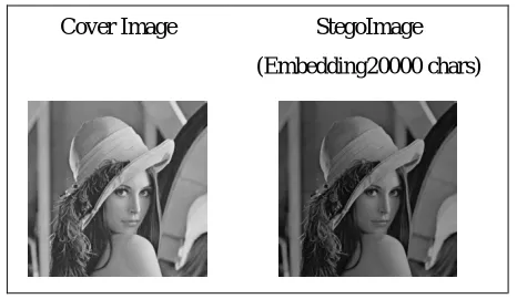
The message deciphered is: “GOD BLESS U CHILD”. Fig.6 shows the cover and stego for this development.
Cover Image StegoImage
(Embedding20000 chars)
[image:8.612.198.412.288.389.2] [image:8.612.190.423.561.696.2]TABLE V
HIDDEN MESSAGE EXTRACTION PROCESS
V.ALGORITHMS
The proposed approach is a spatial domain approach and it has been used in grayscale images. The different algorithms used in
approach are shown below:
A. Algorithm for Data Embedding
1)Divide a grayscale image into 3 by 3 non-overlapping blocks and select two adjacent blocks from the left side simultaneously.
2)Consider the difference between each 8-neighbors of one block in anticlockwise direction with each 8-neighbors of another block in clockwise direction.
3)The no. of bits to be embedded in each of the difference of the value depends on the difference of center pixels of the two adjacent blocks.
4)Convert the difference values into their corresponding binary values.
5)Select a secret message and convert it into its binary form.
6)Map 2-bit or 3-bit or 4-bit of the binary form of secret message in every difference of the neighboring pixels based on intensity value, no. of one’s (in binary), 2nd set-reset and 3rd set-reset bit present in that difference value.
7)Modified difference will be generated. Adjust it in two neighbor pixel pair each belonging from one of two consecutive blocks and obtain the modified blocks.
Difference of pixel intensity values
Pixel Intensity
Value
Binary Form NO.O
F
ONES (BIN)
2nd
SET-RESET
Bit
Extracted 3-Bit
8 - 7 = 1 ODD 00000001 EVEN EVEN 010
10 - 2 = 8 EVEN 00001000 ODD EVEN 001
9 - 4 = 5 ODD 00000101 EVEN ODD 110
9 - 13 = 4 EVEN 00000100 ODD ODD 101
14 - 14 = 0 EVEN 00000000 EVEN EVEN 000
4 - 12 = 8 EVEN 00001000 ODD EVEN 001
10 - 10 = 0 EVEN 00000000 EVEN EVEN 000
8)Repeat the process for all the adjacent blocks and obtain the stego image.
B. Algorithm for Data Extraction
1)Select the stego image and divide into 3 by 3 non-overlapping blocks. Select two adjacent blocks from the left side simultaneously.
2)Consider the difference between each pixel intensity value of one block in anticlockwise direction with each pixel intensity value of another block in clockwise direction.
3)The no. of bits to be extracted from each of the difference of the value depends on the difference of center pixels of the two adjacent blocks.
4)Convert the difference values into their corresponding binary values.
5)Match the binary value of the differences with the properties of its corresponding PMM table and obtain corresponding 2 bits or 3 bits or 4 bits of the binary form of secret message.
6)Arrange the obtained bits in an orderly manner and get the required secret information.
VI.RESULTSANDANALYSIS
In this section the authors have presented experimental results of the proposed method based on two benchmark techniques for
evaluating the hiding performance. First one is the data hiding capacity and the second one is the imperceptibility of the stego
image. The quality of the stego image should be acceptable to human eyes. The experiments have been performed on two
well-known images: Lena and Pepper. The quality of the stego images created by the developed method has been tested by
different qualitative and quantitative similarity metrics. The quantitative values are illustrated in Table.5.
A. Qualitative Similarity Metrics
The quality of stego image produced by the proposed methods and the stego image has been tested thorough statistical parameters
like Mean, Standard Error Mean, Tr Mean, Standard Deviation, Variance, CoefVar, Sum, Sum of Squares, First quartile (Q1),
Median (Q2), Third quartile (Q3), Range, Interquartile (IQR), Mode, N for Mode, Skewness, Kurtosis, MSSD, Covariance etc.
Then examined the relative error for the steganography methods with respect to embedding rate of each methods by calculating the
parameters value. Relative errors are plotted on a graph and it shows that the error rate of developed method is less than the LSB
and PVD method. The quality of the steganography approach is depending upon the relative error graph. When the relative error is
less than or equal to the others method, the performance is better.
B. Mathematical Schemes
stE
Statistical parameters,R
err
Relative ErrorCalculate
E
standE
Average
Average
(
E
st)
Estimate the relative error ....(2)
) (
) (
) (
Average
Average Average
err
E Cover
E Cover E
Stego
R
used in this method.
Plot the
R
errin a graph.Table 6 illustrates the parameter values as well as relative error. In the equation “2”, Stego denotes the statistical parameter values
of LSB, PVD and PMM Variable Bit. Figure 7 shows the graph that shows the relative errors.The details of the tests are discussed
below:
1) Mean: In statistics and probability, the mean [8] is used to denote one measure of the central tendency either of a probability distribution or random variable which is characterized by distribution. For a data set, the mathematical expectation, arithmetic
mean and at times average are used to refer to a central value of a discrete set of numbers: definitely, the sum of the values
divided by the number of values. For a finite population, the population mean of a property is equal to the arithmetic mean of
the given property while considering every member of the population. For example, the population mean height is equal to the
sum of the heights of every individual divided by the total number of individuals. The sample mean may differ from the
population mean, especially for small samples. The law of large numbers dictates that the larger the size of the sample, the
more likely it is that the sample mean will be close to the population mean.
2) Standard Error Mean: The standard error (SE) [9] is the standard deviation of the sampling distribution of a statistic, most commonly of the mean. The term may also be used to refer to an estimate of that standard deviation, derived from a particular
sample used to compute the estimate.
3) Trimmed Mean: A truncated mean or trimmed mean [10] is a statistical measure of central tendency, much like the mean and median. It involves the calculation of the mean after discarding given parts of a probability
distribution or sample at the high and low end, and typically discarding an equal amount of both. This number of points to be
discarded is usually given as a percentage of the total number of points, but may also be given as a fixed number of points.
4) Standard Deviation: In statistics, the standard deviation [11] (SD, also represented by the Greek letter sigma, σ) is a measure that is used to quantify the amount of variation or dispersion of a set of data values. A standard deviation close to 0 indicates
that the data points tend to be very close to the mean (also called the expected value) of the set, while a high standard
deviation indicates that the data points are spread out over a wider range of values.
5) Variance: In probability theory and statistics, variance [12] measures how far a set of numbers is spread out. A variance of zero indicates that all the values are identical. Variance is always non-negative: a small variance indicates that the data points
tend to be very close to the mean (expected value) and hence to each other, while a high variance indicates that the data points
are very spread out around the mean and from each other.
6) Coefficient of Variation: In probability theory and statistics, the coefficient of variation (CV) [13] is a standardized measure of dispersion of a probability distribution or frequency distribution. It is defined as the ratio of the standard deviation to
the mean . It is also known as unitized risk or the variation coefficient. The absolute value of the CV is sometimes known
as relative standard deviation (RSD), which is expressed as a percentage. The coefficient of variation (CV) is defined as the
ratio of the standard deviation to the mean
into four equal groups, each group comprising a quarter of the data. A quartile is a type of quantile. The first quartile (Q1) is
defined as the middle number between the smallest number and the median of the data set. The second quartile (Q2) is the
median of the data. The third quartile (Q3) is the middle value between the median and the highest value of the data set.
In applications of statistics such as epidemiology, sociology and finance, the quartiles of a ranked set of data values are the four
subsets whose boundaries are the three quartile points. Thus an individual item might be described as being "in the upper quartile".
a) First quartile (designated Q1) also called the lower quartile or the 25th percentile (splits off the lowest 25% of data from the
highest 75%)
b) Second quartile (designated Q2) also called the median or the 50th percentile (cuts data set in half)
c) Third quartile (designated Q3) also called the upper quartile or the 75th percentile (splits off the highest 25% of data from the
lowest 75%)
d) Interquartile range (designated IQR) is the difference between the upper and lower quartiles. (IQR = Q3 - Q1)
8) Range: In arithmetic, the range [15] of a set of data is the difference between the largest and smallest values. However, in descriptive statistics, this concept of range has a more complex meaning. The range is the size of the smallest interval
which contains all the data and provides an indication of statistical dispersion. It is measured in the same units as the data.
Since it only depends on two of the observations, it is most useful in representing the dispersion of small data sets.
9) Mode: The mode [16] is the value that appears most often in a set of data. The mode of a discrete probability distribution is the value x at which its probability mass function takes its maximum value. In other words, it is the value that is most likely to
be sampled. The mode of a continuous probability distribution is the value x at which its probability density function has its
maximum value, so, informally speaking, the mode is at the peak.
10) Skewness: In probability theory and statistics, skewness [17] is a measure of the asymmetry of the probability distribution of a real-valued random variable about its mean. The skewness value can be positive or negative, or even undefined. The
qualitative interpretation of the skew is complicated. For a unimodal distribution, negative skew indicates that the tail on the
left side of the probability density function is longer or fatter than the right side – it does not distinguish these shapes.
Conversely, positive skew indicates that the tail on the right side is longer or fatter than the left side. In cases where one tail is
long but the other tail is fat, skewness does not obey a simple rule. For example, a zero value indicates that the tails on both
sides of the mean balance out, which is the case both for a symmetric distribution, and for asymmetric distributions where the
asymmetries even out, such as one tail being long but thin, and the other being short but fat. Further, in multimodal
distributions and discrete distributions, skewness is also difficult to interpret. Importantly, the skewness does not determine
the relationship of mean and median.
11) Kurtosis: In probability theory and statistics, kurtosis [17] (from Greek: κυρτός, kyrtos or kurtos, meaning "curved, arching") is any measure of the "peakedness" of the probability distribution of a real-valued random variable. In a similar way to the
concept of skewness, kurtosisis a descriptor of the shape of a probability distribution and, just as for skewness, there are
different ways of quantifying it for a theoretical distribution and corresponding ways of estimating it from a sample from a
population. There are various interpretations of kurtosis, and of how particular measures should be interpreted; these are
primarily peakedness (width of peak), tail weight, and lack of shoulders (distribution primarily peak and tails, not in between).
two. Two common applications are: Basic Statistics - A common application for the MSSD is a test to determine whether a
sequence of observations is random. In this test, the estimated population variance is compared with MSSD. Control Charts -
MSSD can also be used to estimate the variance for control charts when the subgroup size is 1.
13) Covariance: In probability theory and statistics, covariance [19] is a measure of how much two random variables change together. If the greater values of one variable mainly correspond with the greater values of the other variable, and the same
holds for the smaller values, i.e., the variables tend to show similar behavior, the covariance is positive. In the opposite case,
when the greater values of one variable mainly correspond to the smaller values of the other, i.e., the variables tend to show
opposite behavior, the covariance is negative. The sign of the covariance therefore shows the tendency in the linear
relationship between the variables. The magnitude of the covariance is not easy to interpret. The normalized version of the
covariance, the correlation coefficient, however, shows by its magnitude the strength of the linear relation.
TABLE VI
RELATIVE ERROR OF STATISTICAL PARAMETERS FOR LSB,PVD&PMMVARIABLE BIT
Relative Error Error Change Rate
Embeddi
ng Rate LSB PVD
PMM
Variable Bit LSB PVD
PMM Variable Bit
0.01 0.594135 0.594145 0.594132 - - -
0.02 0.594137 0.594147 0.593864 0.000330457 0.000330452 -0.045127106
0.03 0.594139 0.594149 0.59394 0.000330454 0.000330449 0.012793753
0.04 0.59414 0.59415 0.593941 0.000165365 0.000165362 0.000165417
0.05 0.594141 0.594151 0.593943 0.000248028 0.000248024 0.000248116
0.06 0.594144 0.594154 0.593946 0.000495448 0.00049544 0.000495604
0.07 0.594145 0.594155 0.593996 0.000248109 0.000248104 0.008500794
0.08 0.594147 0.594157 0.593998 0.000248009 0.000248005 0.000248077
0.09 0.594151 0.594161 0.594001 0.000660326 0.000660314 0.000660489
0.10 0.594157 0.594167 0.594008 0.001072732 0.001072714 0.001073002
0.20 0.618186 0.614178 0.60789 4.044193122 3.36791274 2.337099567
0.30 0.643722 0.644226 0.618369 4.130839167 4.892384589 1.723758207
0.40 0.67025 0.671285 0.624742 4.121022483 4.200281168 1.03054472
0.50 0.701124 0.701328 0.633479 4.606251606 4.475347783 1.398625563
0.60 0.730485 0.729378 0.647099 4.187745064 3.99951526 2.149919873
0.70 0.764325 0.759445 0.654036 4.632494072 4.122372437 1.07213002
0.80 0.798682 0.794491 0.661533 4.495126382 4.614706708 1.146205085
0.90 0.833222 0.824524 0.676717 4.324619269 3.780116807 2.295205632
It has been observed that the developed method is robust and secure, which has been verified with the help of relative error graph
and various statistical parameters. Thus the developed method works better than LSB, PVD mechanisms.
C. Quantitative Similarity Metrics
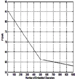
1) Peak Signal-to-Noise Ratio (PSNR): A mathematical extent of image quality is Signal–to-noise ratio (SNR) [20], which is based on the pixel difference between two images [21]. The SNR measure the estimate of Stego image and cover image.
PSNR is shown in equation (3).
Where, S is for the maximum possible pixel value of the image. When the PSNR is greater than 36 DB, the visibility looks same in
[image:14.612.170.432.430.705.2]between the cover and stego image; in that case the HVS is not identifying the changes.
Fig. 8 Graphical representation of PSNR
)
3
...(
...
...
log
10
2
10
MSE
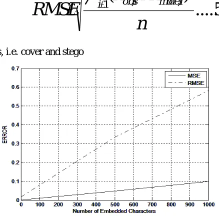
2) Mean Square Error (MSE): It is computed by averaging the squared intensity of the cover and stego image pixels [20]. The equation (4) and fig.9 shows the MSE.
Where NM is the image size (N x M) and e(m,n) is the reconstructed image.
Root Mean Square Error (RMSE): RMSE [22] is a frequently used measure of difference in between Cover and Stego intensity
values. These individual differences called residuals and RMSE aggregate them into a single measure of analytical power. The
RMSE shows in equation (5) and fig.9.
[image:15.612.193.412.250.469.2]Xobsi and Xmodeli are two image vectors, i.e. cover and stego
Fig. 9: Graphical representation of MSE and RMSE
3) Correlations: Pearson’s correlation coefficient [23] is widely used in statistical analysis as well as image processing. Here to apply it in, Cover and Stego image, to see the difference between these two images. The Correlation shows in equation (6) and
fig.10.
The Xi and Yi are the cover image and bar of X and Y are stego image positions.
4) Structural Similarity Index (SSIM): Wang et. al[24], proposed Structural Similarity Index [21] concept between original and distorted image. The Stego and Cover images are divided into blocks of 8 x 8 and converted into vectors. Then two means and
two standard derivations and one covariance value are computed. After that the luminance, contrast and structure comparisons
based on statistical values are computed. Then The SSIM computed between Cover and Stego images. SSIM shows in
equation (7) and fig.10.
)
6
...(
)
(
)
(
)
(
)
(
1 2 1 2 1
n i i n i i ni i i
y
y
x
x
y
y
x
x
r
...
...(
4
)
1
1 0 1 0 2,
M m N nn
m
e
NM
MSE
)
5
...(
)
(
1 2 , ,n
X
X
RMSE
ni obsi modeli
...(
7
)
2
2
2 2 2 2 2 1C
C
Fig. 10 Graphical representation of Correlation and SSIM
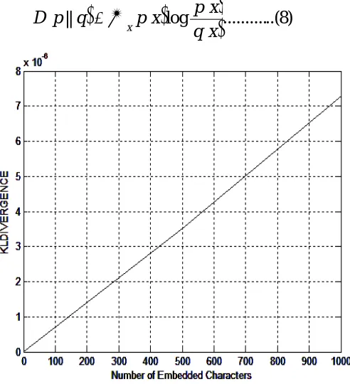
5) KL divergence: With the help of probability density function (PDF) for each Image (cover and stego) estimating the Kullback-Leibler Divergence [25]. KL divergence shows in equation (8) and fig.11.
Fig. 11: Graphical representation of Kullback-Leibler Divergence
...
..(
8
)
log
||
x
x
q
x
p
x
p
q
[image:16.612.178.424.422.692.2]TABLE VII
VARIOUS IMAGE SIMILARITY METRICS FOR THE PROPOSED METHOD
Images Metrics Length of Embedding Character
100 500 1000 10000 15000 20000
Lena 512*512
PSNR 68.5963 61.25872 58.1536 47.3525 45.4913 44.0919
MSE 0.009 0.0486641 0.0995 1.1963 1.8363 2.5345
RMSE 0.1114 0.335352 0.5823 5.6511 8.5742 11.3996
SSIM 1 0.9999976 1 0.9978 0.9968 0.9958
Correlation 1 0.9999826 1 0.9996 0.9993 0.9991
KL divergence 6.81E-07 3.52E-06 7.28E-06 1.12E-04 1.70E-04 2.42E-04
Entropy 7.42E-05 7.42E-05 7.42E-05 7.42E-05 7.42E-05 7.42E-05
Lena 256*256
PSNR 62.4378 54.5582 51.3446 40.0599 N/A N/A
MSE 0.0371 0.2276 0.4771 6.4135 N/A N/A
RMSE 0.1986 0.8059 1.732 18.9569 N/A N/A
SSIM 1 0.9987 0.9962 0.9689 N/A N/A
Correlation 1 1 1 0.9988 N/A N/A
KL divergence 1.76E-06 1.11E-05 2.51E-05 4.41E-04 N/A N/A
Entropy 0 0 0 0 N/A N/A
Lena 128*128
PSNR 54.9411 47.3213 43.9515 N/A N/A N/A
MSE 0.2084 1.2049 2.6177 N/A N/A N/A
RMSE 0.5378 2.594 5.3829 N/A N/A N/A
SSIM 0.9997 0.9944 0.9903 N/A N/A N/A
Correlation 1 0.9998 0.9995 N/A N/A N/A
KL divergence 1.06E-05 7.35E-05 1.49E-04 N/A N/A N/A
Entropy 0 0 0 N/A N/A N/A
TABLE VIII
COMPARISON OF EMBEDDING CAPACITY
IMAGE IMAGE
SIZE PVD GLM
AHMAD
et al.
PMM(2
bit)
Proposed
Method
Lena 512*512 50960 32768 40017 45340 58254
256*256 ** 8192 10007 10012 14564
128*128 ** 2048 2493 2393 3641
Pepper 512*512 50685 32768 39034 46592 58254
256*256 ** 8192 9767 11694 14564
TABLE IX
COMPARISON OF PSNR VALUES BETWEEN PMM4-BIT AND PROPOSED METHOD
Image
PSNR
Character length PMM(4 bit) Proposed Method
Lena512*512
100 63.4131 68.5963
500 59.309 61.2563
1000 56.309 58.1536
10000 47.7562 50.0027
15000 44.5811 47.3525
20000 41.3445 44.0919
6) Entropy: Entropy [26] is a measure of the uncertainty associated with a random variable. Here, a 'message' means a specific realization of the random variable. The equation (9) and fig.12 shows it.
Where, S is the entropy and T is the uniform thermodynamic temperature of a closed system divided into an incremental
reversible transfer of heat into that system (dQ).
Fig.12 Graphical representation of Entropy
VII. COMPARISONWITHEXISTINGMETHODS
A comparative study of the proposed methods with some other existing methods like PVD, GLM and the methods proposed by
Ahmad T et al. is discussed in this section. TABLE VIIIshows the comparison of different methodologies with the help of
embedding capacity.
TABLE IX shows the comparison of PSNR values of PMM (4 bit) and the proposed method.
VIII.CONCLUSION
A new and efficient steganography method for embedding secret messages in grayscale images has been proposed here. The
experimental results through qualitative and quantitative similarity metrics clearly indicate that the embedding capability of this
)
9
...(
.
method is much higher than both conventional PMM and PVD methods. In future authors will work on biometric steganography
using the variable embedding technique using PMM two, three and four bit simultaneously.
REFERENCES
[1] Abbas Cheddad., Joan Condel., Kevin Curran., Paul McKevitt. "Digital image steganography: Survey and analysis of current methods Signal Processing" 90,
2010,pp. 727– 752.
[2] Y. Hsiao., C.C. Chang. and C.-S. Chan., "Finding optimal least significant-bit substitution in image hiding by dynamic programming strategy." Pattern
Recognition, 36:1583–1595, 2003.
[3] Potdar V and Chang E., "Gray Level Modification Steganography for secret communication" In IEEE International Conference on Industrial Informations,pages
355-368, berlin, germany,2004.
[4] H.C. Wu, N.I. Wu, C.S. Tsai and M.S. Hwang, "Image steganographic scheme based on pixel value differencing and LSB replacement method", IEEE
Proceedings on Vision, Image and Signal processing, Vol. 152, No. 5,pp. 611-615, 2005.
[5] P Huang., K.C. Chang., C.P Chang and T.M Tu., "A novel image steganography method using tri-way pixel value differencing". Journal of Multimedia, 3, 2008.
[6] Bhattacharyya, S. and Sanyal, G. "Hiding Data in Images Using Pixel Mapping Method (PMM)". SAM'10 - 9th annual Conference on Security and Management
under The 2010 World Congress in Computer Science, Computer Engineering, and Applied Computing held on July 12-15, 2010, USA.
[7] Bhattacharyya, S., Kumar, L. and Sanyal, G. "A Novel approach of Data Hiding Using Pixel Mapping Method (PMM)". International Journal of Computer
Science and Information Security (IJCSIS-ISSN 1947-5500) , Volume. 8 , N0. 4 , JULY 2010,Page No -207-214.
[8] Feller, William (1950). Introduction to Probability Theory and its Applications, Vol I. Wiley. p. 221. ISBN 0471257087
[9] Everitt, B.S. (2003), The Cambridge Dictionary of Statistics, CUP. ISBN 0-521-81099-X.
[10] Arulmozhi, G., Statistics For Management, 2nd Edition, Tata McGraw-Hill Education, 2009, p. 458.
[11] Bland J.M.,Altman, D.G. (1996). "Statistics notes: measurement error." (PDF). Bmj, 312(7047), 1654. Retrieved22 November 2013.
[12] Yuli Zhang,HuaiyuWu,Lei Cheng. (June 2012). Some new deformation formulas about variance and covariance. Proceedings of 4th International Conference on
Modelling, Identification and Control(ICMIC2012). pp. 987–992.
[13] Broverman, Samuel A. (2001). Actex study manual, Course 1, Examination of the Society of Actuaries, Exam 1 of the Casualty Actuarial Society (2001 ed. ed.).
Winsted, CT: Actex Publications. p. 104. ISBN 9781566983969. Retrieved 7 June 2014.
[14] Hyndman, Rob J., Fan, Yanan (November 1996). "Sample quantiles in statistical packages". American Statistician 50 (4): 361–365. doi:10.2307/2684934.
[15] George Woodbury (2001). An Introduction to Statistics. Cengage Learning. p. 74. ISBN 0534377556.
[16] Hippel, Paul T. von (2005). "Mean, Median, and Skew: Correcting a Textbook Rule". J. of Statistics Education 13 (2).
[17] Joanes, D. N., Gill, C. A. (1998). "Comparing measures of sample skewness and kurtosis". Journal of the Royal Statistical Society (Series D): The Statistician 47
(1): 183–189.
[18] Neumann, J. von., Kent,R. H., Bellinson, H. R. and Hart, B. I., “The Mean Square Successive Difference” The Annals of Mathematical Statistics, Vol. 12, No. 2
(Jun., 1941), pp. 153-162.
[19] Yuli Zhang., Huaiyu Wu,Lei Cheng (June 2012). Some new deformation formulas about variance and covariance. Proceedings of 4th International Conference on
Modelling, Identification and Control(ICMIC2012). pp. 987–992.
[20] Yusra A. Y. Al-Najjar, Dr. Der Chen Soong, "Comparison of Image Quality Assessment: PSNR, HVS, SSIM, UIQI", International Journal of Scientific &
[21] A. L. M. Jean-Bernard Martens, "Image dissimilarity", Signal Processing, vol. 70, no. 3, pp. 155-176, 1998.
[22] Lehmann, E. L., Casella, George. (1998). "Theory of Point Estimation (2nd ed.)". New York: Springer. ISBN 0-387-98502-6.
[23] J.L.Rodgers, J.L. and W.A.Nicewander, "Thirteen Ways to Look at the Correlation Coefficient", American Statistician 42, 59-66 (1995).
[24] A. C. B. Zhou Wang, "A Universal Image Quality Index," IEEE SIGNAL PROCESSING LETTERS, vol. 9, pp. 81-84, 2002.
[25] Pedro J. Moreno., Purdy Ho., NunoVasconcelos. "A Kullback-Leibler Divergence Based Kernel for SVM Classification in Multimedia Applications" Conference:
Neural Information Processing Systems - NIPS , 2003