Comparative Analysis of Frequent Pattern Matching Based On Apriori & Enhanced Algorithms

Comparative Analysis of Frequent Pattern

Matching Based On Apriori & Enhanced

Algorithms

Bhukya Krishna1, Dr. Geetanjali Amaravathi2 1

Associate Prof, Dept of CSE, CMR Technical Campus, Kandlakoya, Medchal, Telangana, India

2

Professor, Dept of CSE, Madhav University, Abhu Road, Sirohi, Rajasthan, India

Abstract : Data mining strategies have been broadly utilized for removing non-paltry data from such huge measures of data. It is helpful in numerous applications like key basic leadership, monetary conjecture, and medicinal conclusion and so forth. Data mining can be connected either as a elucidating or as a prescient device. Affiliation manage mining is one of the functionalities of data mining. This postulation proposes a couple of strategies for moving forward affiliation govern mining, affiliation administer covering up, and post mining. The way toward creating affiliation rules includes the errand of finding the set of all the successive thing sets and creating promising standards. This issue can be understood by mining Maximal Frequent Sets (MFS) alone. Despite the fact that data mining has a ton of benefits, it has a couple of bad marks moreover. Delicate data contained in the database might be brought out by the data mining devices. Distinctive methodologies are being utilized to shroud the delicate data. It is watched that a large portion of the concealing algorithms in the current writing, work at the exchanges level to conceal some touchy data. This is a tedious stride in the concealing procedure. In this theory, two new procedures have been proposed to lessen the time multifaceted nature of the concealing procedure. A major organization may have various branches spread crosswise over various areas. Handling of data from these branches turns into a colossal undertaking when multitudinous exchanges occur. Neighborhood mining may likewise create a lot of standards. Further, it is most certainly not for all intents and purposes feasible for every single nearby data sources to be of a similar size.

Keywords: About Apriori, Candidate item set, enhanced Apriori, Frequent patterns, Support, Confidence, Association Rule, Apriori Algorithm, soft set.

I. INTRODUCTION A. Data Mining

Figure1.1 Data Mining Process (KDD)

The part of data mining (KDD) is essential in a large number of the fields, for example, examination of market wicker container, grouping, and so forth. In the event that discussion about data mining, the most imperative part introduced by visit thing set which visit thing set which is utilized to discover the connection between's the different kind of the field that is shown in the database. Revelation of incessant thing set is finished by affiliation rules. Retail location likewise utilizes the idea of affiliation rules for overseeing showcasing, publicizing, and blunders that are exhibited in the media transmission arrange.

The relationship among the things is finished by affiliation rules. All sort of connection between things is completely in light of the Co-event of thing. The Knowledge find in data can accomplish by following strides:

1) Data Cleaning: In this progression data that is insignificant and if clamor is available in database then both unimportant and boisterous data is expelled from database.

2) Data Integration: In this progression the diverse sorts of data and different data sources are participated in a typical source. 3) Data Selection: In this stage, the application dissects that what data, what sort of data is recovered from the gathering of data. 4) Data Transformation: In this stage chosen data is changed into precise frame for the method of Data mining.

5) Data Mining: This is the essential stride in which the method used to extricate the pattern is cunning.

6) Pattern Evaluation: In this progression extremely required patterns speak to colleagues in view of measures parameters.

7) Knowledge Representation: This is the last stride in which learning is outwardly spoken to the client. Information portrayals utilize perception strategies to help in understanding of client and taking the yield of the KDD.

B. Frequent Pattern Mining

Frequent patterns will be patterns that show up frequently in a data set. Finding frequent patterns assumes a fundamental part in mining associations, connections, and numerous other intriguing connections among data. For case, an arrangement of things, for example, glue and brush, which show up frequently together in an exchange data set, is a frequent thing set. Consider the situation, for example, purchasing initial a PC, at that point a data card, and then a pen drive, and if this pattern happens frequently in a shopping history database, at that point that pattern is a frequent pattern. A substructure can allude to various auxiliary structures, for example, sub diagrams, sub trees, or sub cross sections, which might be consolidated with thing sets or sub arrangements. Frequent pattern-mining looks for repeating connections in a given data set. Market wicker bin examination is the soonest type of frequent pattern mining for association rules.

C. Frequent Pattern Mining Methods

There are various methods for mining frequent item sets. They are

2) Apriori Algorithm: Apriori algorithm is utilized to discover visit item sets. A portion of the applications are recorded underneath:

a) Cancer treatment

b) Cross selling in retail industry c) Online book store

d) Student placement e) Diabetics detection f) Games

D. Mining FI without Candidate Generation

Visit design development, or FP-development mines the entire arrangement of successive item sets without creating the applicant, and receives a partition and-vanquish procedure. FP development holds the item set affiliation information by packing the database speaking to visit things into an incessant example tree, or FP-tree. It at that point partitions the database that is in packed shape into an arrangement of restrictive databases; each related with one regular thing or example piece and mines every database independently. Just the related data sets should be inspected for each example part, bringing about the diminishment in the size of the data to be looked, development of examples being analyzed and seek cost have been decreased. At the point when the database size is huge, it is now and then unreasonable to build a primary memory based FP-tree and an option approach is to segment the database into an arrangement of anticipated databases, and afterward develop a FP-tree and mine the incessant examples from each anticipated database. In the event that its FP-tree can't fit in fundamental memory, this procedure can be recursively connected to any anticipated database for getting the successive examples.

E. Mining FI using Vertical Data Format

In Vertical data organize, utilizing thing Tidset design data can be spoken to where thing determines the thing name and Tidset is the arrangement of transaction identifiers containing the thing. Utilizing vertical data design, frequent itemsets can be mined. To begin with, change the on a level plane designed data into the vertical arranged data by filtering the data set once. The length of the TID set of the item set is the support number of the item set. Beginning with k = 1, the Frequent k-Item sets can be utilized to build the hopeful (k+1) itemsets in view of the Apriori property. The frequent itemsets can be mined by convergence of the Tidset of the frequent k-itemsets to figure the Tidset of the comparing (k+1)-itemsets. This procedure is rehashed, in each time k increased by 1, until no frequent itemsets or applicant itemsets can be found. The benefit of this strategy is that there is no compelling reason to check the database to discover the support of (k+1) –itemsets, on the grounds that the tidset of every k-item set is having the entire information required for numbering such support. The disservice of this strategy is, that if the TID sets be very long, at that point it will consume considerable memory room and more calculation time for crossing the long sets.

F. Mining Closed Frequent Item set

Utilizing mining process, shut frequent itemsets can be mined by pruning the pursuit space. Pruning methodologies incorporate the thing blending, sub-itemset pruning and thing skipping. In thing blending, if each transaction containing a frequent itemset An additionally contains an itemset B however no appropriate superset of B, at that point AUB shapes a frequent shut itemset and no compelling reason to scan for any itemset containing A yet not B. In thing skipping, at each level of profundity initially mining of shut itemsets, there will be a prefix itemset a related with a header table and an anticipated database. On the off chance that a neighborhood frequent thing p has a similar support in a few header tables at various levels, prune p from the header tables at more elevated amounts.

G. Association Rule Mining

II. FREQUENT PATTERNS MINING EVOLUTION

Frequent examples are thing sets, sub successions, or substructures that show up in a data set that fulfills the client indicated least support check with recurrence at the very least a client determined edge. Agrawal et al. [1] proposed a productive algorithm that creates all the association administers between the things in the customer transaction database and this algorithm consolidates novel estimation, support administration and pruning techniques. This algorithm is connected on sales data of an extensive retailing organization and viability of the algorithm has been demonstrated. Agrawal et al [2] proposed two algorithms Apriori and AprioriTid for tackling the issue of mining frequent examples, and afterward joined both of these algorithms. The Apriori and AprioriTid algorithms produce the hopeful thing sets to be numbered in a go by utilizing just the itemsets discovered huge in the past pass not considering the transactions in the database. This system brings about era of a substantially more modest number of competitor itemsets. The Apriori Tid algorithm has the property that the database is not utilized at all to count the support of applicant itemsets after the primary pass. Srikant et al [3] presents the mining of summed up association rules from an expansive database of transactions, which indicates the association between the data things accessible in the transaction.

III. IMPROVED TECHNIQUE FOR RETRIEVING FREQUENT PATTERNS

Jiawei Han et al [4], proposed FP-development, for mining the total arrangement of frequent examples, the productivity of mining is accomplished with three techniques: a substantial database is compacted into an exceptionally dense significantly littler data structure, which maintains a strategic distance from expensive, rehashed database checks, FP-tree-based mining receives an example section development strategy to keep away from the exorbitant era of countless sets. Cheng-Yue Chang et al.,[11] investigate another algorithm called Segmented Progressive Filter which portion the database into databases such that things in each sub-database will have either the basic beginning time or the basic closure time. For each sub-sub-database, SPF dynamically channels hopeful 2-itemsets with combined sifting edges either forward or in reverse in time. This component permits SPF of embracing the output decrease strategy by producing all applicant k-itemsets (k >2) from competitor 2-itemsets specifically.

A. Techniques for Association Rule Mining

Mining association decides implies that, given a database of sales transactions, to discover all associations among the things with the end goal that the nearness of a few things in a transaction will suggest the nearness of different things in a similar transaction. The mining of association rules is the issue of finding substantial itemsets where an expansive itemset is a gathering of things that show up in an adequate number of transactions whose check fulfills the client determined least support tally. A hash based algorithm is created by Jong soo et al.,[13], which lessens the database size, so that applicant itemset produced at each progression will be diminished, so that computational cost is decreased. Wei et al., [21] proposed Association Rule Growth algorithm, which at the same time find frequent itemsets and association controls in an expansive database. Algorithm was investigated by producing the association run and it performs effectively.

B. Mining Frequent Patterns Using GA

Maritine et al., [11] proposed a hereditary algorithm way to deal with take out the powerless thing sets to support the survival of the best ones by working on the huge population. By utilizing hereditary based methodologies of having wellness work, best association control is additionally found. Cunrong et al., [18] recommended a hereditary algorithm based association run the show. It is more proficient than Apriori algorithm, and the time take for producing the association lead is less, with the goal that effectiveness is expanded. Hereditary algorithm performs worldwide pursuit and adapt preferred to attribute communication over the covetous administer enlistment algorithms for the discovery of abnormal state forecast rules utilized as a part of data mining. Wei et al., [32] display a strategy for similar association rules mining utilizing Genetic Network Programming (GNP) with attributes gathering system so as to reveal association administers between various datasets. GNP is a developmental approach which can advance itself and could locate the ideal arrangements. The inspiration of the similar association rules mining technique is to utilize the data mining way to deal with check whether at least two databases are utilized rather than one, and locate the shrouded relations among them. The proposed strategy measures the significance of association leads by utilizing the outright contrast of confidences among various databases and can get various intriguing tenets.

C. Mining Association Rules

books. The discovered patterns are the set of books most frequently bought together by the customers. An example could be that “40% of the people who buy Chetan Bhagat’s The 3 Mistakes of My Life also buy Five Point Someone”. The store can use this knowledge for promotions, shelf placement, etc. There are many potential application areas for association rule technology, which includes catalog design, store layout, customer segmentation, telecommunication alarm diagnosis, and so on. The task of discovering all frequent associations in very large databases is quite challenging. The search space is exponential in the number of database attributes and with millions of database objects the problem of I/O minimization becomes paramount. However, most current approaches are iterative in nature, requiring multiple database scans, which is clearly very expensive. Also, most approaches use very complicated internal data structures which have poor locality and add additional space and computation overheads. The goal is to minimize all of these limitations.

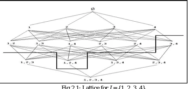
1) Traversing the Search Space: As clarified, we have to discover all itemsets that fulfill minsup. For down to earth applications taking a gander at all subsets of I is bound to disappointment by the colossal inquiry space. Actually, straightly developing number of things still suggests an exponential developing number of itemsets that should be considered. For instance, consider the situation where the quantity of things is 20, (n=20). The quantity of itemsets of size 1 wills be20. The quantity of itemsets of size 2 will be20 et cetera. Consequently the aggregate number of itemsets that could be framed for n=20, would be 20+ 20 +…+ 20 =2, in the event that we incorporate the invalid set. Therefore the quantity of itemsets that should be sought in the dataset would be 2 = 1048576. The essential approach utilized by algorithms that discover affiliation rules is to recognize visit and non-visit itemsets so the inquiry space can be confined. For the exceptional case I = {1, 2, 3, 4} we picture the hunt space that structures a cross section in Figure 1 [9]. The successive itemsets are situated in the upper piece of the figure though the occasional ones are situated in the lower part. Albeit unequivocal help esteems for each of the itemsets are not determined, it is expected that the intense fringe isolates the regular from the rare itemsets. The presence of such a fringe is autonomous of a specific database D and minsup. Its reality is exclusively ensured by the descending conclusion property of itemset bolster. The fundamental guideline of the normal algorithms is to utilize this fringe to productively prune the inquiry space. When the fringe is discovered, we can confine ourselves on determining the help estimations of the itemsets over the outskirt and to disregard the itemsets underneath.

Fig 2.1: Lattice for I = {1, 2, 3, 4}

design {TID: itemset}, where TID is exchange id and itemset is the arrangement of things contained in the exchange. Then again, mining can likewise be performed with data parceled in vertical data design. {Item: TID-set}. Brief presentation of algorithms that help vertical data arrange is additionally given.

3) 1AIS: The AIS calculation was first distributed calculation created to produce all huge itemsets in an exchange database [1]. It concentrated on the improvement of databases with vital usefulness to prepare choice help questions. This calculation was focused to find subjective guidelines. This system is constrained to just a single thing in the resulting. The AIS calculation makes various ignores the whole database. Amid each pass, it checks all exchanges. In the main pass, it numbers the help of individual things and figures out which of them are extensive or visit in the database. Vast itemsets of each pass are stretched out to create applicant itemsets. Subsequent to checking an exchange, the normal itemsets between huge itemsets of the past pass and things of this exchange are resolved. Consider the arrangement of exchanges in Table 1 as an example dataset to represent the working of AIS calculation. Figure 2 demonstrates the era of applicant itemsets and the successive itemsets by the AIS calculation. Least Support in the illustration is considered as half, i.e. 2 exchanges. As observed from the Figure 2, itemset {4} is absent in L1 as its number in exchanges is 1 (not exactly minsup). The competitor itemset of size 2, C2 is found by broadening L1 with singular exchanges. Expanding L1 with first exchange creates {1, 3}, {1, 4}, {3, 4}. Additionally L1 is stretched out with different exchanges to get C2 as appeared in Figure 2. From C2, L2 is found as those itemsets whose number is more noteworthy than the base help. As found in the Figure {1, 3}, {2, 3}, {2, 5}, {3, 5} have tallies more noteworthy than or equivalent to least help and they frame L2. C3 is then created in the comparative path by expanding L2 with all exchanges. {2, 3, 5} is the main itemset that has bolster number equivalent to the base help and thus it moves toward becoming L3. Expanding L3 with exchanges brings about an invalid set so the calculation ends here.

Transaction ID (TID) Transactions Elements

100 {1, 3, 4} 200 {2, 3, 5} 300 {1, 2, 3, 5}

400 {2, 5}

Table 2.1 Transaction ID (TID)

4) SETM: The SETM calculation proposed in [20] and was inspired by the craving to utilize SQL to ascertain substantial itemsets [34]. In this calculation every individual from the set substantial itemsets is in the frame <TID, itemset> where TID is the one of a kind identifier of an exchange. Likewise, every individual from the arrangement of competitor itemsets is in the shape <TID, itemset>. Like the AIS calculation, the SETM calculation makes various ignores the database. In the main pass, it numbers the help of individual things and figures out which of them are visit in the database. At that point, it produces the applicant itemsets by broadening extensive itemsets of the past pass. Also, SETM recollects the TIDs of the producing exchanges with the competitor itemsets. The social union join operation can be utilized to produce applicant itemsets [30]. Producing competitor sets, the SETM calculation spares a duplicate of the hopeful itemsets together with TID of the creating exchange in a successive way. A short time later, the competitor itemsets are arranged on itemsets, and little itemsets are erased by utilizing a conglomeration work. On the off chance that the database is in arranged request on the premise of TID, extensive itemsets contained in an exchange in the following cruise are acquired by arranging on TID. Thusly a few passes are made on the database. At the point when not any more expansive itemsets are discovered, the calculation ends. The fundamental hindrance of this calculation is because of the quantity of applicant sets [3]. Since for every applicant itemset there is a TID related with it, it requires more space to store a lare number of TIDs. Moreover, when the help of a competitor itemset is numbered toward the finish of the pass, is not in requested design. Along these lines, again arranging is required on itemsets. At that point, the applicant itemsets are pruned by disposing of the competitor itemsets which don't fulfill the help imperative. Another sort on TID is fundamental for the coming about set ( ). Subsequently, can be utilized for creating applicant itemsets in the following pass. Figure 3 demonstrates the generation of hopeful itemsets and the continuous itemsets by the SETM calculation considering the dataset given in Table 1. Least Support in the case is considered as half, i.e. 2 exchanges.

property that any subset of a vast itemset must be an expansive itemset. Likewise, it is accepted that things inside an itemset are kept in lexicographic request. The key contrasts of this calculation from the AIS and SETM algorithms are the method for creating competitor itemsets for numbering. As said before, in both AIS and SETM algorithms, the regular itemsets between expansive itemsets of the past pass and things of an exchange are acquired. These normal itemsets are reached out with other individual things in the exchange to create hopeful itemsets. Be that as it may, those individual things may not be huge. As we realize that a superset of one huge itemset and a little itemset will bring about a little itemset, these techniques create excessively numerous applicant itemsets which end up being little. The Apriori calculation tends to this essential issue. The Apriori creates the competitor itemsets by joining the vast itemsets of the past pass and erasing those subsets which are little in the past go without considering the exchanges in the database. By just considering extensive itemsets of the past pass, the quantity of hopeful huge itemsets is fundamentally lessened. Since its origin which don't fulfill the help requirement. Another sort on TID is essential for the coming about set. The Apriori calculation created by [2] is an extraordinary accomplishment in the historical backdrop of mining affiliation rules [11]. It is by a wide margin the most understood affiliation control calculation. This method utilizes the property that any subset of a vast itemset must be an expansive itemset. Likewise, it is accepted that things inside an itemset are kept in lexicographic request. The key contrasts of this calculation from the AIS and SETM algorithms are the method for creating competitor itemsets for numbering. As said before, in both AIS and SETM algorithms, the regular itemsets between expansive itemsets of the past pass and things of an exchange are acquired. These normal itemsets are reached out with other individual things in the exchange to create hopeful itemsets. Be that as it may, those individual things may not be huge. As we realize that a superset of one huge itemset and a little itemset will bring about a little itemset, these techniques create excessively numerous applicant itemsets which end up being little. The Apriori calculation tends to this essential issue. The Apriori creates the competitor itemsets by joining the vast itemsets of the past pass and erasing those subsets which are little in the past go without considering the exchanges in the database. By just considering extensive itemsets of the past pass, the quantity of hopeful huge itemsets is fundamentally lessened. Since its origin which don't fulfill the help requirement. Another sort on TID is essential for the coming about set. Thereafter, can be utilized for creating applicant itemsets in the following pass. Figure 3 demonstrates the generation of applicant itemsets and the regular itemsets by the SETM calculation considering the dataset given in Table 1. Least Support in the illustration is considered as half, i.e. 2 exchanges., numerous different algorithms [5, 6, 7, 9, 22, 26, 27] have risen that enhance the run-time, I/O and versatility execution of the first Apriori calculation by different productive methods for pruning the itemset look space and numbering the hopeful events in expansive databases. The Apriori algorithm [2] is given in Figure 4.

6) FP-GROWTH: FP-Growth [6] is a calculation to mine regular examples and it is a non-competitor generation calculation utilizing an exceptional structure FP-tree. FP-tree is an expansion of prefix tree structure. Just incessant things have hubs in the tree. Every hub contains the things name and its recurrence. The ways from the root to the leaves are orchestrated as indicated by the help of the things, with the recurrence of each parent more prominent than or equivalent to the whole of its kids' recurrence. The development of the FP-tree requires two data examines. In the primary output, the help of everything is found. In the second output, things with exchanges are arranged in the plummeting request as per the help of things. Hubs with a similar mark are associated with a thing join. The thing join is utilized to encourage visit design mining. Moreover, each FP-tree has a header that contains every incessant thing and pointers to the start of their separate thing join.

IV. MINING FREQUENT ITEMSETS USING VERTICAL DATA LAYOUT

The algorithms talked about before create visit itemsets from an arrangement of exchanges in level data organize {TID: itemset}, where TID is the exchange id and itemset is the arrangement of things contained in that exchange. On the other hand mining can be performed with data introduced in vertical data design {item: Tidset}. M. J Zaki [32] proposed six proficient algorithms for the revelation of successive itemsets. The algorithms to be specific Éclat, Max Éclat, Clique, Max Clique, Top Down and ArpClique use the auxiliary properties of the regular itemsets to encourage quick revelation. The things are sorted out into a subset grid look space, which is disintegrated into little autonomous lumps or subtleties which can be unraveled in memory. Proficient cross section traversal techniques utilized immediately distinguished throughout the entire the regular itemsets and their subsets if required.

A. Parallel and Distributed Algorithms

computational work may bring about restrictively vast runtimes on single processors. Along these lines, it is basic to outline productive parallel algorithms to do the assignment. Another explanation behind outlining parallel algorithms originates from the way that numerous exchange databases are as of now accessible in parallel databases or they are disseminated at various destinations in the first place. The cost of presenting to them all to one site or one PC for serial disclosure of affiliation guidelines might be restrictively costly.

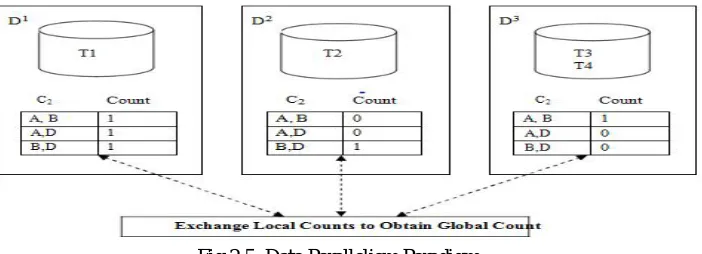
Fig 2.5: Data Parallelism Paradigm

1) PDM: Parallel Data Mining) [30] is a modification of CD with inclusion of the direct hashing technique proposed in [29]. The hash technique is used to prune some candidates in the next pass. It is especially useful for the second pass, as Apriori doesn’t have any pruning in generating C2 from L1. In the first pass, in addition to counting all 1-itemsets, PDM maintains a hash table

for storing the counts of the 2-itemsets. Note that in the hash table we don’t need to store the 2-itemsets themselves but only the count for each bucket. For example, if suppose {A, B} and {C} are large items in the hash table for the 2-itemsets the bucket containing {AB, AD} turns out to be small (the count for this bucket is less than the minimum support count). PDM will not generate AB as a size 2 candidate by the hash technique, while Apriori will generate AB as a candidate for the second pass, as no information about 2-itemsets can be obtained in the first pass. For this communication, in the kth pass, PDM needs to exchange the local counts in the hash table for k+1-itemsets in addition to the local counts of the candidate k-itemsets.

2) IDD: IDD (Intelligent Data Distribution) is a change over DD [24]. It segments the competitors over the processors in view of the primary thing of the hopefuls, that is, the applicants with a similar first thing will be apportioned into a similar parcel. Along these lines, every processor needs to check just the subsets which start with one of the things doled out to the processor. This lessens the repetitive calculation in DD, concerning DD every processor needs to check all subsets of every exchange, which presents a considerable measure of excess calculation. To accomplish a heap adjusted dispersion of the competitors, it utilizes a container pressing method to segment the hopefuls, that is, it initially figures for everything the quantity of applicants that start with the specific thing, and after that it utilizes a canister pressing calculation to dole out the things to the applicant segments to such an extent that the quantity of hopefuls in each segment is equivalent. It additionally embraces ring design to decrease correspondence overhead, that is, it utilizes no concurrent point to point correspondence between neighbors in the ring as opposed to broadcasting.

3) HPA: HPA (Hash-based Parallel mining of Association rules) utilizes a hashing procedure to appropriate the possibility to various processors [38], i.e., every processor utilizes a similar hash capacity to figure the applicants disseminated to it. In tallying, it moves the subset itemsets of the exchanges to their goal processors by a similar hash strategy, rather than moving the database allotments among the processors. This suggests one subset itemset of an exchange just goes to one processor rather than n. HPA was additionally enhanced by utilizing the skew taking care of system [31] [21]. The skew taking care of is to copy a fewapplicants if there is accessible fundamental memory in every processor, with the goal that the workload of every processor is more adjusted.

V. FUZZY APPROACH IN MINING

additionally incorporates the different conditions of truth in the middle. For instance, the aftereffect of an examination between two things could be not "tall" or "short" but rather ".38 of height."

Fuzzy logic appears to be nearer to the way our brains work. The total data shape various incomplete certainties which total further nto higher realities which thus, when certain edges are surpassed, because certain further outcomes, for example, engine response. A comparative sort of process is utilized as a part of manufactured PC neural network and master systems.

As frequent data itemsets mining are very important in mining the Association rules. Therefore there are various techniques are proposed for generating frequent itemsets so that association rules are mined efficiently.

VI. CONCLUSION

The proposed algorithms, reduces number of scans of transactional database while generating Lk. Execution time also improved when compared with Apriori and Apriori1. This represents that Apriori2 takes less time in generating frequent patterns. If the value of support is increased then the number of scans also gets decreased (for generating L1 number of scans decreases and for L2 and above the number of scans always remains zero). The proposed algorithm fits for larger transactional databases because the proposed algorithm doesn’t scan transactional database while generating Lk (k>1). It looks into only transactional ids. This proposed algorithmsare apt for problems in areas like marketing, whether, health care etc.The proposed algorithm for mining association rule, decreases pruning operations of candidate 2-itemsets, thereby saving time and increase efficiency. It optimizes subset operation, through the transaction tag to speed up support calculations. The experimental results obtained from tests show that proposed system outperforms original one efficiently. The current mining methods require users to define one or more parameters before their execution; however, most of them do not mention how users can adjust these parameters online while they are running. It is not feasible for users to wait until a mining algorithm to stop before they can reset the parameters. This is because it may take a long time for the algorithm to finish due to the continuous arrival and huge amount of data. For further improvement, we may consider either let the users adjust online or let the mining algorithm auto-adjust most of the key parameters in association rule mining, such as support, confidence and error rate.

REFERENCES

[1] J. Han, and M. Kamber, “Data Mining: Concepts and Techniques”, Morgan Kaufmann Publishers, 2000.

[2] J. D. Holt, and S. M. Chung, “Efficient Mining of Association Rules in Text Databases”, in CIKM'99, Nov 1999, Kansas City, USA, pp. 234242.

[3] B. Mobasher, N. Jain, E.H. Han, and J. Srivastava, “Web Mining: Pattern Discovery from World Wide Web Transactions”, Department of Computer Science, University of Minnesota, March 1996, Technical Report TR96-050.

[4] C. Ordonez, and E. Omiecinski, “Discovering Association Rules Based on Image Content”, IEEE Advances in Digital Libraries, 1999.

[5] R. Agrawal, T. Imielinski, and A. Swami, “Mining association rules between sets of items in large databases”, in ACM SIGMOD International Conference on Management of Data, May 1993, Washington, USA, pp. 207216.

[7] R. Bayardo, and R. Agrawal, “Mining the most interesting rules”, in 5th International Conference on Knowledge Discovery and Data Mining, San Diego, August 1999, California, USA, pp. 145154.

[8] J. Hipp, U. Güntzer, and U. Grimmer, “Integrating association rule mining algorithms with relational database systems”, in 3rd International Conference on Enterprise Information Systems, July 2001, Setúbal, Portugal, pp. 130137.

[9] R. Ng, L. S. Lakshmanan, J. Han, and T. Mah, “Exploratory mining via constrained frequent set queries”, in ACM-SIGMOD International Conference on Management of Data, June 1999, Philadelphia, PA, USA, pp. 556558.

[10] Y. Guizhen, “The complexity of mining maximal frequent itemsets and maximal frequent patterns”, in ACM SIGKDD International Conference on Knowledge Discovery and Data Mining , August 2004, Seattle, WA, USA, pp. 343353.

[11] L. Klemetinen, H. Mannila, P. Ronkainen, et al., “Finding interesting rules from large sets of discovered association rules”, in Third International Conference on Information and Knowledge Management, 1994, Gaithersburg, USA, pp. 401407.

[12] J. S. Park, M.S. Chen, and P.S. Yu, “An Effective HashBased Algorithm for Mining Association Rules”, in ACM SIGMOD International Conference on Management of Data, 1995, San Jose, CA, USA, pp. 175186.

[13] H. Toivonen, “Sampling large databases for association rules”, in 22nd International Conference on Very Large Data Bases, 1996, pp. 134–145.

[14] P. Kotásek, and J. Zendulka, “Comparison of Three Mining Algorithms for Association Rules”, in 34th Spring International Conference on Modelling and Simulation of Systems, 2000, Workshop Proceedings Information Systems Modelling, pp. 8590.

[15] J. Han, J. Pei, and Y. Yin, “Mining frequent patterns Candidate generation”, in ACMSIGMOD International Management of Data, 2000, Dallas, TX.

[16] F. H. AL-Zawaidah, Y. H. Jbara, and A. L. Marwan, “An Improved Algorithm for Mining Association Rules in Large Databases”, International Journal on Natural Language Computing , Vol. 1, No. 7, 2011, pp. 311-316.

[17] J. Han, M. Kamber, “Data Mining: Concepts and Techniques”, Morgan Kaufmann Publishers, Book, 2000.

[18] Mohammed Al-Maolegi1, and Bassam Arkok2, “International Journal on Natural Language Computing”, Vol. 3, No.1, February 2014. [19] Agrawal R, Srikant R (1994) Fast algorithms for mining association rules. In: Proceedings of the 20th VLDB conference, pp 487–499 [20] Ahmed S, Coenen F, Leng PH (2006) Tree-based partitioning of date for association rule mining. KnowlInfSyst 10(3):315–331 [21] Banerjee A, Merugu S, Dhillon I, Ghosh J (2005) Clustering with Bregman divergences. J Mach Learn Res 6:1705–1749 [22] Bezdek JC, Chuah SK, Leep D (1986) Generalized k-nearest neighbor rules. Fuzzy Sets Syst18(3):237–256.

[23] Bloch DA, Olshen RA, Walker MG (2002) Risk estimation for classification trees. J Comput Graph Stat 11:263–288 [24] Bonchi F, Lucchese C (2006) On condensed representations of constrained frequent patterns. KnowlInfSyst 9(2):180–201

[25] Breiman L (1968) Probability theory. Addison-Wesley, Reading. Republished (1991) in Classics of mathematics. SIAM, Philadelphia [26] Breiman L (1999) Prediction games and arcing classifiers. Neural Comput 11(7):1493–1517

[27] Breiman L, Friedman JH, Olshen RA, Stone CJ (1984) Classification and regression trees. Wadsworth, Belmont [28] Brin S, Page L (1998) The anatomy of a large-scale hyper textualWeb Search Sngine. Comput Networks 30(1–7):107–117 [29] Chen JR (2007) Making clustering in delay-vector space meaningful. Know lInfSyst 11(3):369–385

[30] CheungDW,HanJ,NgV,WongCY(1996) Maintenance of discovered association rules in large databases:an incremental updating technique. In: Proceedings of the ACM SIGMOD international conference on management of data, pp. 13–23

[31] Chi Y, Wang H, Yu PS, Muntz RR (2006) Catch the moment: maintaining closed frequent itemsets over a data stream sliding window. KnowlInfSyst 10(3):265–294

[32] Cost S, Salzberg S (1993) A weighted nearest neighbor algorithm for learning with symbolic features. Mach Learn 10:57.78 (PEBLS: Parallel Examplar-Based Learning System)

[33] Cover T, Hart P (1967) Nearest neighbor pattern classification. IEEE Trans Inform Theory 13(1):21–27

[34] Dasarathy BV (ed) (1991) Nearest neighbor (NN) norms: NN pattern classification techniques. IEEE Computer Society Press