The effect of empirical-statistical correction of intensity-dependent
model errors on the temperature climate change signal
A. Gobiet1,2, M. Suklitsch2, and G. Heinrich1,a
1Wegener Center for Climate and Global Change (WegCenter), University of Graz, Graz, Austria
2Central Institute for Meteorology and Geodynamics (ZAMG), Department of forecasting models, Vienna, Austria anow at: Department of Geography and Regional Science, University of Graz, Graz, Austria
Correspondence to: A. Gobiet ([email protected])
Received: 25 March 2015 – Published in Hydrol. Earth Syst. Sci. Discuss.: 16 June 2015 Revised: 4 September 2015 – Accepted: 10 September 2015 – Published: 6 October 2015
Abstract. This study discusses the effect of empirical-statistical bias correction methods like quantile mapping (QM) on the temperature change signals of climate simula-tions. We show that QM regionally alters the mean tempera-ture climate change signal (CCS) derived from the ENSEM-BLES multi-model data set by up to 15 %. Such modifica-tion is currently strongly discussed and is often regarded as deficiency of bias correction methods. However, an analyti-cal analysis reveals that this modification corresponds to the effect of intensity-dependent model errors on the CCS. Such errors cause, if uncorrected, biases in the CCS. QM removes these intensity-dependent errors and can therefore potentially lead to an improved CCS. A similar analysis as for the multi-model mean CCS has been conducted for the variance of CCSs in the multi-model ensemble. It shows that this indica-tor for model uncertainty is artificially inflated by intensity-dependent model errors. Therefore, QM also has the poten-tial to serve as an empirical constraint on model uncertainty in climate projections. However, any improvement of sim-ulated CCSs by empirical-statistical bias correction methods can only be realized if the model error characteristics are suf-ficiently time-invariant.
1 Introduction
Society is increasingly demanding reliable projections of fu-ture climate change to analyze adaptation options and costs, to explore climate change mitigation benefits, and to sup-port political decisions. Such climate projections are usu-ally generated with general circulation models (GCMs) of
rather coarse spatial resolution, which are refined by dy-namical or statistical downscaling methods (e.g., Giorgi and Mearns, 1991; Fowler et al., 2007). Currently, an increasing number of climate change impact investigations rely on dy-namical downscaling methods, i.e., the use of regional cli-mate models (RCMs, e.g., Giorgi and Mearns, 1991, 1999; Wang et al., 2004; Rummukainen, 2010). However, even the newest generation of RCMs features considerable systematic errors (e.g., Kotlarski et al., 2014), which complicates the di-rect application of RCM results in climate change impact re-search. RCM output is therefore usually post-processed with empirical-statistical “bias correction” methods (e.g., Déqué, 2007; Themeßl et al., 2011) before it is used as input for impact models, such as hydrological models. Bias correc-tion methods have been demonstrated to successfully reduce systematic model errors (i.e., the difference between histor-ical model output and meteorologhistor-ical observations), but the knowledge about how they influence the climate change sig-nal (CCS; i.e., the long-term average difference between a future and a past climate simulation) is very limited so far.
A relation between model errors and CCS has been dis-cussed by Christensen et al. (2008), who found that monthly temperature errors of RCMs over Europe often depend on the observed monthly mean temperature and that in warmer months, errors are often larger than in colder months (or vice versa). Such “intensity-dependent” errors can be shown to alter the temperature CCS (Christensen et al., 2008; The-meßl et al., 2012; Boberg and Christensen, 2012).
op-eration over Europe in some regions and seasons, and found a lower summer temperature CCS in eastern Europe as well as a higher winter temperature CCS in Scandinavia after bias correction with QM. Currently, such modifications are often regarded as an undesired deficiency of bias correction meth-ods (e.g., Hempel et al., 2013). However, Maurer and Pierce (2014) recently claimed that QM may have no negative effect on the quality of the CCS and demonstrated that QM does not deteriorate the multi-model mean precipitation CCS in a GCM ensemble.
In this paper we go a step further and argue that, under the assumption of time-invariant model error characteristics, the modification of the CCS by QM can be interpreted as improvement, rather than as deterioration, since it is capable of mitigating intensity-dependent model errors. To support this hypothesis, we develop a linearized analytical descrip-tion of the effect of intensity-dependent model errors on the CCS. This framework allows the impact of such errors to be investigated, not only on the multi-model mean CCSs in an ensemble of climate simulations, but also on the inter-model variability, which is often used as a measure of uncertainty in climate projections (e.g., Hawkins and Sutton, 2009, 2011; Prein et al., 2011). Furthermore, we compare the analytical correction of the CCS to the correction by QM.
In Sect. 2, the QM method is described and its effect on the temperature CCS of the ENSEMBLES multi-model data set is demonstrated. In Sect. 3, the error characteris-tics of the ENSEMBLES models are analyzed, and in Sect. 4 we present an analytical formulation of intensity-dependent model errors and their effects on the CCS. In Sect. 5 these effects are compared to the effects of QM on CCSs, and in Sect. 6 a summary is given and conclusions are drawn.
2 Quantile mapping and its effect on climate change signals over Europe
2.1 Quantile mapping
The basic assumption of QM is that model errors depend on the value of the simulated variable. This concept of intensity-dependent errors is a rough simplification of actual model error characteristics, since model errors are not only influ-enced by the local value of the simulated variable. How-ever, we will demonstrate that errors and local values cor-relate well in many cases (Sect. 3). The concept is simple yet powerful, since it separates, e.g., cold from hot regimes, or drizzling from heavy precipitation regimes and therefore ac-counts for potentially very different model errors under the associated regimes. It should be emphasized that intensity-dependent model errors are equivalent to a misrepresentation of variability, i.e., to differences between the observed and modeled width of the density distribution. Figure 1 demon-strates that intensity-dependent error characteristics with a positive slope correspond to overestimated variability, if the
model error is defined as the difference between the inverse modeled and observed empirical cumulative density func-tions (ECDF). Similarly, a negative error slope corresponds to underestimation of variability.
QM is a distribution-based bias correction method (e.g., Panofsky and Brier, 1958; Wood et al., 2004) that maps a modeled historical ECDF to an observed ECDF, with the mapping function shown in Fig. 1c for an artificial example. It is a well-established method to prepare climate model out-put as inout-put for hydrological models (e.g., Déqué, 2007; Ma-raun et al., 2010; Themeßl et al., 2011) and has been success-fully applied to the sum of daily precipitation and air tem-perature of RCMs and GCMs by Dobler and Ahrens (2008), Piani et al. (2010a, b), Dosio and Parulo (2011), Dosio et al. (2012), Maurer and Pierce (2014) and others. Further-more, Themeßl et al. (2011) showed for daily precipitation sums that QM outperforms six other prominent bias correc-tion techniques.
In our study, a non-parametric version of QM is used (The-meßl et al., 2011, 2012; Wilcke et al., 2013), as suggested by Gudmundsson et al. (2012). The ECDFs are constructed from 930 values for each day of the year based on modeled and observed data of a 30-year reference period (1961–1990) and a 31-day moving window, centered on the day under con-sideration. Our implementation of QM is not restricted to the range of observed values in the reference period, since the correction is extrapolated beyond the calibration range by using the correction term of the highest and lowest quan-tile, respectively. Please note, that this implies constant (not intensity-dependent) error characteristics outside the calibra-tion range. As discussed by Bellprat et al. (2013), such con-stant errors at high temperatures outside the calibration range may be more realistic in many cases than a linear extrapola-tion.
Figure 1. Intensity-dependent model errors of a model that overestimates daily temperature variability (artificial data). (a) Modeled (red, standard deviation of 5◦C) and observed (green, standard deviation of 4◦C) empirical density functions; (b) modeled (red) and observed (green) ECDFs; (c) model error at different modeled values.
al., 2010a; Themeßl et al., 2012; Gudmundsson et al., 2012; Wilcke et al., 2013), or for future periods using a pseudo-reality approach (Maraun, 2012). Furthermore, Teutschbein and Seibert (2013) show that correction methods like QM perform better under non-stationary conditions than widely used linear transformations or the delta-change approaches. This gives confidence that empirical-statistical bias correc-tion with QM is useful not only for historical simulacorrec-tions, but also, though with degraded performance, for future cli-mate simulations. However, in a strict interpretation, the re-sults and conclusions of this study are only valid under the assumption of time-invariant model errors and it is still sub-ject to further investigation to determine the severity of this restriction. Although such investigation is outside the scope of our study, we want to mention that the new centennial re-analyses of ECMWF (ERA-20C) and NOAA-CIRES (V2c) offer a promising new test bed for the investigation of the long-term stability of model error characteristics.
2.2 Model and observational data
We apply QM to a set of 15 GCM-driven regional climate simulations for Europe from the ENSEMBLES multi-model data set (van der Linden and Mitchell, 2009). The ENSEM-BLES models are operated on a 25 km grid and reach until 2100. In the following, we show the results for daily mean temperature, but the analysis of daily minimum and maxi-mum temperatures gives very similar results. The application of our analysis to other parameters like, e.g., precipitation is basically straight forward, but the linearization applied in Sect. 4 can be expected to be less appropriate for precipita-tion than for temperature. Further investigaprecipita-tion is needed to fully reveal the effect of QM on the precipitation CCS. The major motivation for focusing on temperature here is its rel-atively simple error characteristic and its significant climate trend, which facilitates the demonstration of the effect of QM on the CCS.
As observational reference, the ENSEMBLES gridded ob-servational data set (E-OBS, Haylock et al., 2008) is used.
It is a European land-only daily high-resolution (25 km grid spacing) data set for five meteorological parameters, includ-ing daily mean temperature.
2.3 The effect of QM on the CCS in ENSEMBLES
Subsequently, we show the effect of QM on the multi-model mean CCS and on the standard deviation of CCSs for the pe-riods 2021–2050 and 2070–2099, both compared with the reference period 1971–2000. In Fig. 2 the spatial patterns of the difference between the uncorrected and the corrected multi-model mean temperature CCS is shown for different seasons in the middle (left) and end (right) of the 21st cen-tury. In the end of the century, differences exceed+0.5 K in summer (JJA) in larger parts of southeastern Europe, France, and the Iberian Peninsula and −0.5 K in larger regions in Scandinavia, which roughly corresponds to 15 % of the un-corrected CCS. These results are consistent with the analyses of Boberg and Christensen (2012) and Dosio et al. (2012) and indicate that summer warming in southeastern Europe is projected to be less severe, and warming in Scandinavia is projected to be more severe, after bias correction with QM. However, the differences remain in the order of 10 % of the uncorrected CCS and the basic pattern of temperature change is not strongly altered by QM.
Figure 3 shows the spatial pattern of the difference be-tween the uncorrected and the corrected standard deviation of CCSs as a measure of model uncertainty. In most regions, model uncertainty is larger in the uncorrected model ensem-ble (orange colors), particularly in regions where the CCS is overestimated (see Fig. 2). The overestimation locally peaks at 0.5 K. However, in some regions (e.g., Scandinavia) and periods (e.g., late 21st century winter) model uncertainty is smaller in the uncorrected model ensemble, locally peaking at about−0.4 K.
Figure 2. Differences between uncorrected and corrected (QM) multi-model mean temperature CCS. The reference period is 1971–2000. The left panels refer to CCSs in the mid-21st century (2021–2050), the right panels to the end of the 21st century (2070–2099). Blue colors indicate areas where the uncorrected model is colder than the corrected model; red colors vice versa.
Figure 3. Differences between uncorrected and corrected (QM) multi-model standard deviation. The reference period is 1971–2000. The left panels refer to CCSs in the mid-21st century (2021–2050), the right panels to the end of the 21st century (2070–2099). Blue colors indicate areas where the uncorrected ensemble features a smaller standard deviation; orange colors vice versa.
3 Intensity-dependent model errors in the ENSEMBLES multi-model data set
Since intensity-dependent model errors are the main suspects which cause the demonstrated effect of QM on the CCS, we investigate whether such errors exist in the ENSEMBLES RCMs. Due to their contrasting error characteristics, two of the RCMs are discussed in more detail: the HadRM3Q3 (driven by the HadCM3Q3 global climate model) operated by the Hadley Centre (HC), and the RCA (driven by run 3 of the ECHAM5 global climate model) operated by the Swedish Meteorological Service (SMHI). Since model error charac-teristics are known to be regionally very variable, Europe is separated into eight subregions following Rockel and Woth
(2007), which are marked in Figs. 2 and 3: the British Islands (BI), France (FR), central Europe (ME), Scandinavia (SC), Iberian Peninsula (IP), Mediterranean (MD), Alps (AL) and eastern Europe (EA).
[image:4.612.49.547.305.486.2]Figure 4. Temperature error characteristics (model minus observation) of the HC (left panels) and SMHI (right panels) RCMs in eight subregions of Europe (sub-panels) and each month of the year.
each subregion and each month of the year. Figure 4 exem-plarily shows the daily temperature error characteristics of the HC and SMHI models.
Both models are affected by strongly intensity-dependent errors, but the error characteristics of the two models dif-fer substantially. While the HC model features positive error slopes (up to 0.5) in most seasons and regions, the SMHI model has mainly negative slopes (up to−0.7). Both models are rather extreme examples within the ENSEMBLES multi-model data set and most other multi-models feature smaller slopes of about+/−0.1 (Figs. S1 to S8 in the Supplement).
In order to analyze whether such single-model error slopes cancel out in the multi-model ensemble, the ensemble aver-age error characteristics (bold lines) in SC and EA are shown in Fig. 5 together with those of all 15 individual models (light lines). In SC, a considerable negative multi-model average slope exists in most parts of the year (minimum in July). Con-trarily, positive slopes can be found in EA in summer (max-imum in July). Several other regions, like AL, feature only minor multi-model average slopes, but in turn larger slope variability (see Figs. S9 to S12).
4 Analytical description of the effect of
intensity-dependent model errors on the CCS Having shown and quantified the intensity-dependence of model errors in the ENSEMBLES multi-model data set, we subsequently give a simplified analytical description to high-light the mechanism of how such errors act on the CCS in a multi-model ensemble.
4.1 CCS of a single climate simulation
Letyji be the value of a meteorological variable (e.g., tem-perature, precipitation sum, or any other simulated variable) on dayj simulated by modeli.yi is the 30-year average for a specific time of the year, e.g., for a month or a season. It can be expressed as a combination of the observed average valuexand the deviation of the model from this value due to errors (yie) and due to natural and model internal variability (yvi):yi=x+yei+yvi. The CCS1yi (1yi =yfuturei −ypasti ) can then be written as
1yi=1x+1yei+1yvi. (1)
1xdenotes the deterministic part of the error-free CCS,1yei the effect of model errors, and1yvi the random effect of in-ternal variability. In many studies, the model error term is ne-glected (“delta-change approach”), since errors are expected to be time-invariant and to cancel out in the CCS. We demon-strate that this is not the case, even for time-invariant error characteristics, if they are intensity-dependent and the CCS is non-zero. The daily intensity-dependent errors can be writ-ten as a function of the meteorological variable under consid-eration:yei,j=f (yji). For the sake of simplicity, we assume a linear error function with a constant biasbi, error slopesi, and residualεij:
yei,j=bi+siyij+εij. (2)
Figure 5. Temperature error characteristics (modeled minus observed) of the ENSEMBLES models in SC (left panels) and EA (right panels). The light lines show the error characteristics of the individual models, the bold line shows the ensemble average. The number in the lower right corner of each panel denotes multi-model average error slope.
Averaging over 30 years, taking the difference between a future and a past period, and neglecting the residual, yields the linearized effect of the intensity-dependent model error on the CCS:
1yei=si1yi. (3)
The bias cancels out, since it is assumed to be time-invariant and not intensity-dependent. From Eqs. (1) and (3) the simu-lated CCS can be written as
1yi=1x+1y i v
1−si . (4)
Equation (4) shows that intensity-dependent model errors lead to a modeled CCS that is proportional to the error-free CCS (1x+1yvi) and a factor determined by the error slope (1/(1−si)). Figure 6a illustrates this effect in relative terms: positive error slopes lead to an exaggeration of the error-free CCS and negative slopes dampen it, but to a smaller extent. For example, for slopes of 0.1 and −0.1 the error would amount to about 11 and −9 %, respectively. The depicted range of error slopes from−0.7 to 0.5 has been selected ac-cording to temperature error slopes found in the ENSEM-BLES multi-model data set (see Sect. 5).
4.2 Multi-model mean CCS
For a multi-model ensemble, the ensemble mean CCS and the multi-model variance of the CCS is relevant. To derive the effect of intensity-dependent errors on these quantities, the error slope can be written as the sum of the ensemble mean error slope (s) and a model-specific residuum error slope (s0i). Combining this separation with the expanded form of
Figure 6. (a) Effect of the error slope on the single-model CCS. (b) Effect of the error slope on the multi-model mean CCS. Black line: covariance term of 0 K; blue lines: covariance term of−0.02 K; pink lines: covariance term of+0.21 K. The lightest colors corre-spond to an error-free CCS of 1 K, the darkest colors to a CCS of 4 K.
Eq. (4) yields
1yi=1x+s+s0i1yi+1yvi. (5) Accordingly, the multi-model mean CCS is
1yi=1x+s1yi+covs0i
, 1yi. (6)
[image:6.612.307.548.328.441.2]like in the single-model case, and secondly the covariance term, which adds an offset. Figure 6b visualizes the corre-sponding error in the CCS in relative terms: positive multi-model mean error slopes lead to an exaggeration of the CCS, and negative slopes dampen it, just like in the single-model case (black line). The depicted range of multi-model error slopes from−0.16 to+0.13 has been selected according to the multi-model mean temperature error slopes of the EN-SEMBLES multi-model data set (see Sect. 5). Positive and negative covariance terms create positive and negative off-sets, respectively. Following Eq. (3), it can be expected that single-model error slopes and CCSs are generally positively correlated and that the covariance term is consequently pos-itive. The depicted range of covariance terms corresponds to values found in the analysis of temperature errors of the EN-SEMBLES multi-model data set, ranging from−0.02 (blue colors) to+0.21 (pink colors) (Sect. 5), and confirms this ex-pectation. The absolute effect of the covariance term (Eq. 7) is independent from the error-free CCS and thus gets smaller with higher CCS in relative terms, which is indicated by lighter (small CCS) and darker colors (large CCS).
4.3 Variance of CCSs in a multi-model ensemble The effect of intensity-dependent errors on the second im-portant quantity in a multi-model ensemble, the variance of CCSs (which is often interpreted as a measure of uncer-tainty), can be described with the linearized model as well. Using Eqs. (5) and (6), the variance can be expressed as
var(1yi)=1 n
n X
i=1 h
1yi−1yii2=1 n
n X
i=1 h
s1yi−1yi
+s0i1yi+1yvi−covs0i, 1yi i2. (8)
Expanding and simplifying Eq. (8) gives (see the Supplement for a detailed derivation)
var(1yi)=var(1yvi)+s2var(1yi)+var(s0i1yi)
+2scov(1yi, s0i1yi). (9)
Since var(1yvi) is the effect of natural variability, it can be interpreted as the variance of an error-free model ensemble. Compared to that, the variance of a model ensemble with intensity-dependent errors is always exaggerated by a posi-tive offsets2var(1yi). For example, an ensemble mean error slope of±0.1 results in about 1 % bias in variance. In addi-tion, the positive additive term var(s0i1yi), which represents
covariance term can counterbalance the otherwise positive terms, so all terms of Eq. (9) are quantified and analyzed for the ENSEMBLES multi-model ensemble in Sect. 5. 4.4 Linearized correction
The linearized error characterization leads to a simple way to correct the CCS of single models following Eq. (3), the model mean CCS following Eq. (6), and the multi-model variance of CCS following Eq. (9). Error slopes, cli-mate change signals, their variability, and their covariance are calculated based on the comparison of historical sim-ulations with observations and applied to results of future simulations. Such correction assumes not only a linear error-slope, but also time-invariant error characteristics. The lin-early corrected multi-model mean temperature CCS is listed in Table 1 (1xLC) and the variance of the CCSs in Table 2
(var(1x)LC). They are discussed in the following section.
5 Correction of the CCS and its uncertainty
In Table 1 the terms contributing to errors in the multi-model mean CCS (see Eq. 6) are listed for all subregions and sea-sons. Multi-model mean error slopes (s) are mostly nega-tive in DJF and MAM, mostly posinega-tive in JJA and SON, and range from −0.16 in SC in MAM to 0.13 in EA in JJA. Accordingly, they inflate (positive slopes) or dampen (negative slopes) the CCS, depending on season and subre-gion. The errors stemming from the slope term (s 1y) range from −0.25 to 0.20 K in the mid-century and from −0.57 to 0.45 K at the end of the century. Contrary, the covariance term (cov(s0i, 1yi)) is, with very few exceptions, positive and increases the CCS. It amounts 0.04 K on average, ranges from−0.02 to 0.21 K in both periods, but usually does not exceed 0.10 K. Compared to the slope term, the covariance term is smaller in most cases, but cannot be neglected, as it sometimes equals or even exceeds the slope term. Table 1 also lists the uncorrected (1y) and corrected multi-model mean CCS (linearized correction (LC):1xLC; quantile
map-ping:1xQM) for each season and subregion. The difference
Table 1. Multi-model mean temperature error slopes (s), multi-model mean CCSs (1yi), covariance error terms (cov(s0i, 1yi)), linearly corrected CCSs (1xLC), and non-linearly corrected CCSs (1xQM) for the periods 2021–2050 (left) and 2070–2099 (right) (K).
Region Season s Mid-century (2021–2050) End of the century (2070–2099)
1yi s1yi cov(s0i, 1yi) 1x
LC 1xQM 1yi s1yi cov(s0i, 1yi) 1xLC 1xQM
BI
DJF 0.07 1.05 0.06 0.03 0.96 0.97 2.18 0.14 −0.01 2.05 2.05
MAM −0.16 0.94 −0.16 0.03 1.06 0.99 2.08 −0.35 0.04 2.40 2.23
JJA −0.15 0.94 −0.15 0.06 1.03 1.02 2.31 −0.37 0.09 2.59 2.48
SON 0.02 1.10 0.02 0.02 1.06 1.11 2.47 0.04 0.02 2.41 2.50
FR
DJF −0.03 1.31 −0.04 0.03 1.33 1.33 2.54 −0.09 −0.02 2.65 2.65
MAM −0.07 1.03 −0.07 0.04 1.07 1.09 2.40 −0.16 0.05 2.52 2.53
JJA 0.08 1.37 0.10 0.13 1.15 1.22 3.68 0.28 0.21 3.19 3.37
SON 0.00 1.22 0.00 0.01 1.21 1.15 3.08 −0.01 0.02 3.07 2.96
ME
DJF −0.03 1.49 −0.04 0.03 1.50 1.50 3.01 −0.09 −0.01 3.11 3.14
MAM −0.06 1.01 −0.06 0.01 1.06 1.04 2.35 −0.13 0.01 2.47 2.42
JJA 0.05 1.14 0.05 0.07 1.01 1.08 3.00 0.13 0.10 2.77 2.85
SON 0.02 1.23 0.02 0.01 1.20 1.16 3.01 0.05 0.01 2.95 2.82
SC
DJF −0.06 1.84 −0.12 0.06 1.90 1.99 4.37 −0.30 0.02 4.64 4.80
MAM −0.16 1.57 −0.27 0.07 1.77 1.62 3.59 −0.64 0.05 4.17 3.85
JJA −0.14 1.25 −0.20 0.01 1.44 1.46 2.68 −0.42 0.01 3.09 3.11
SON −0.10 1.66 −0.17 0.02 1.81 1.76 3.56 −0.38 0.02 3.91 3.81
IP
DJF −0.04 1.24 −0.04 0.01 1.27 1.21 2.33 −0.08 0.00 2.41 2.34
MAM −0.04 1.22 −0.05 0.05 1.22 1.25 3.11 −0.12 0.07 3.16 3.22
JJA 0.04 1.66 0.06 0.05 1.55 1.58 4.44 0.17 0.06 4.21 4.32
SON 0.00 1.45 0.01 0.02 1.42 1.41 3.51 0.01 0.04 3.45 3.48
MD
DJF −0.08 1.36 −0.11 0.02 1.45 1.38 2.78 −0.24 0.02 3.00 2.96
MAM −0.05 1.27 −0.07 0.05 1.29 1.33 3.04 −0.17 0.08 3.14 3.20
JJA 0.00 1.85 0.00 0.05 1.80 1.87 4.35 0.01 0.09 4.26 4.47
SON −0.04 1.44 −0.06 0.03 1.47 1.38 3.41 −0.14 0.05 3.50 3.40
AL
DJF −0.02 1.54 −0.03 0.03 1.55 1.40 3.15 −0.07 −0.01 3.22 2.95
MAM −0.06 1.29 −0.09 0.03 1.35 1.37 3.00 −0.21 0.04 3.17 3.24
JJA 0.02 1.58 0.03 0.06 1.48 1.57 4.10 0.09 0.10 3.91 4.08
SON 0.05 1.35 0.06 0.01 1.28 1.24 3.37 0.15 0.02 3.20 3.16
EA
DJF −0.04 1.70 −0.06 0.03 1.73 1.67 3.39 −0.12 0.00 3.52 3.44
MAM −0.01 1.19 −0.01 0.02 1.18 1.18 2.79 −0.02 0.03 2.78 2.80
JJA 0.13 1.54 0.17 0.08 1.29 1.34 3.52 0.40 0.12 3.00 3.07
SON 0.03 1.41 0.04 0.01 1.36 1.29 3.23 0.09 0.02 3.12 2.97
Mean −0.03 1.35 −0.04 0.04 1.35 1.34 3.12 −0.08 0.04 3.16 3.15
differences are found in the later period, when QM often indi-cates smaller errors than LC. This can be probably explained by the fact that LC extrapolates intensity-dependent errors, while our implementation of QM keeps the error constant outside the calibration range (see Sect. 2.1). This dampens the error slope under severe warming (i.e., at the end of the 21st century) when daily temperatures outside the calibra-tion range frequently occur. Further discrepancies between QM and LC can be explained by the linear approximation of LC. Both correction methods agree that the uncorrected CCS is regionally biased up to+0.5 K in EA and FR in summer and about−0.5 K in SC. The qualitative agreement of QM with LC can be interpreted as a confirmation that the correc-tion of intensity-dependent errors is the main reason of the modification of the CCS by QM.
T able 2. Multi-model v ariance of the temperature CCSs (v ar (1y
i)),
error terms of the v ariance ( s 2v ar (1y
i),
v
ar
(s
0
i 1y i),
and 2 s co v (1y i, s 0 i 1y i)),
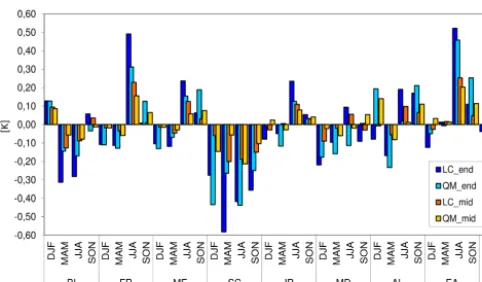
Figure 7. Estimated errors in the multi-model mean CCS due to intensity-dependent model errors. The reference period is 1971– 2000. The orange colors refer to CCSs in the mid-21st century (2021–2050), the blue colors to the end of the 21st century (2070– 2099). Light colors correspond to the estimation of the error by QM, dark colors to LC.
period). The average covariance term 2scov(1yi, s0i1yi)is very small in both periods (−0.002 and+0.002 K2, respec-tively) and ranges from −0.028 to 0.136 K2. In summary, the positive variability term, var(s0i1yi), dominates and is mostly even enhanced by the covariance term. This leads to a general overestimation of ensemble variance.
Table 2 also lists the uncorrected (var(1yi)) and corrected variance of the CCSs in the multi-model ensemble (LC: var(1xLC); QM: var(1xQM))for each season and subregion.
The average difference between uncorrected and corrected variance over all seasons and regions does not cancel out as in the case of the mean CCS, but amounts on average to 17 % in the case of LC and to 12 % in the case of QM. This demon-strates that time-invariant intensity-dependent errors inflate model uncertainty in multi-model ensembles. In Fig. 8 this error is expressed as standard deviation, which is overesti-mated by up to 0.4 K at the end of the century. This is par-ticularly the case in regions where the mean CCS is overes-timated like in EA in summer. However, the two correction methods disagree in some cases as, e.g., in SC in winter at the end of the century. These discrepancies are currently not fully understood and require further analysis. They could, e.g., be caused by the linearity assumption of LC, by the constant (not intensity-dependent) correction outside the calibration range of QM, or by time-variant model errors.
6 Summary and conclusions
[image:10.612.306.550.66.207.2]The knowledge about the influence of empirical-statistical bias correction methods like QM on the CCS of climate sim-ulations is very limited so far. For the ENSEMBLES multi-model data set it has been demonstrated that QM damp-ens projected summer warming in southeastern Europe and France by about 0.5 K and enhances projected warming in
Figure 8. Estimated errors in the multi-model standard deviation of the temperature CCS due to intensity-dependent model errors. The reference period is 1971–2000. The orange colors refer to CCSs until the mid-21st century (2021–2050), the blue colors until the end of the 21st century (2070–2099). Light colors correspond to the estimation of the error by QM, dark colors to LC.
Scandinavia by about the same amount. This corresponds to about 15 % of the uncorrected CCS. Such modification is cur-rently strongly discussed and is often regarded as deficiency of bias correction methods. However, we argue that under the assumption of time-invariant model errors, QM should gen-erally lead to an improvement of the simulated CCS rather than deterioration.
To support this hypothesis, we analytically formulated the effect of intensity-dependent model errors on the CCS and showed that they erroneously modify the CCS. Positive er-ror slopes lead to an exaggeration of the CCS and negative slopes dampen it. This is the case for a single model’s CCS as well as for the multi-model mean CCS in a model en-semble, which is additionally exaggerated by high variabil-ity amongst the single model’s CCSs. A comparison of this analytically determined error and the effect of QM on the mean CCS in the ENSEMBLES multi-model data set leads to largely similar results. This confirms that the effect of QM on the CCS is mainly caused by the correction of intensity-dependent errors and that such modification can be regarded as improvement, if roughly time-invariant model error char-acteristics can be assumed.
mate change. The improvements primarily refer to the mean CCS, but also an empirical constraint on uncertainty in multi-model climate projections seems to be feasible. A restriction to these results is the fact that any potential improvement can only be realized if the assumption of time-invariant model er-ror characteristics sufficiently holds. It is still subject to fur-ther investigation to determine the severity of this restriction.
The Supplement related to this article is available online at doi:10.5194/hess-19-4055-2015-supplement.
Author contributions. A. Gobiet is responsible for the general con-cept and conduction of the study, for the analytical description pre-sented in Sect. 4, for the interpretation of the results and for writing the text. M. Suklitsch contributed the analysis of the error character-istics of the ENSEMBLES models and G. Heinrich the analysis of the effect of QM on the climate change signal in the ENSEMBLES data set. Both were also involved in the discussion of the results and contributed to parts of the text.
Acknowledgements. This study was partly funded by the EU FP7 projects ACQWA (grant agreement 212250) and IMPACT2C (grant agreement 282746). We acknowledge the E-OBS data set from the EU-FP6 project ENSEMBLES (http://ensembles-eu.metoffice.com) and the data providers in the ECA&D project (http://www.ecad.eu). The ENSEMBLES data used in this work was funded by the EU FP6 Integrated Project ENSEMBLES (Contract number 505539) whose support is gratefully acknowledged.
Edited by: L. Oudin
References
Bellprat, O., Kotlarski, S., Lüthi, D., and Schär, C.: Physical con-straints for temperature biases in climate models, Geophys. Res. Lett., 40, 4042–4047, doi:10.1002/grl.50737, 2013.
Boberg, F. and Christensen, J. H.: Overestimation of Mediterranean summer temperature projections due to model deficiencies, Na-ture Climate Change, 2, 433–436, doi:10.1038/nclimate1454, 2012.
Christensen, J. H., Boberg, F., Christensen, O. B., and Lucas-Picher, P.: On the need for bias correction of regional climate change projections of temperature and precipitation, Geophys. Res. Lett., 35, L20709, doi:10.1029/2008GL035694, 2008.
high-resolution climate change projections for use by impact models: evaluation on the present climate, J. Geophys. Res., 116, D16106, doi:10.1029/2011JD015934, 2011.
Dosio, A., Paruolo, P., and Rojas, R.: Bias correction of the EN-SEMBLES high resolution climate change projections for use by impact models: analysis of the climate change signal, J. Geophys. Res., 117, D17110, doi:10.1029/2012JD017968, 2012.
Eden, J. M., Widmann, M., Grawe, D., and Rast, S.: Skill, correc-tion, and downscaling of GCM-simulated precipitacorrec-tion, J. Cli-mate, 25, 3970–3984, doi:10.1175/JCLI-D-11-00254.1, 2012. Fowler, H. J., Blenkinsop, S., and Tebaldi, C.: Linking climate
change modelling to impacts studies: recent advances in down-scaling techniques for hydrological modelling, Int. J. Climatol., 27, 1547–1578, doi:10.1002/joc.1556, 2007.
Giorgi, F. and Mearns, L. O.: Approaches to the simulation of re-gional climate change: a review, Rev. Geophys., 29, 191–216, doi:10.1029/90RG02636, 1991.
Giorgi, F. and Mearns, L. O.: Introduction to special section: re-gional climate modeling revisited, J. Geophys. Res., 104, 6335– 6352, doi:10.1029/98JD02072, 1999.
Gudmundsson, L., Bremnes, J. B., Haugen, J. E., and Engen-Skaugen, T.: Technical Note: Downscaling RCM precipitation to the station scale using statistical transformations – a com-parison of methods, Hydrol. Earth Syst. Sci., 16, 3383–3390, doi:10.5194/hess-16-3383-2012, 2012.
Hawkins, E. and Sutton, R.: The potential to narrow uncertainty in regional climate predictions, B. Am. Meteorol. Soc., 90, 1095– 1107, doi:10.1175/2009BAMS2607.1, 2009.
Hawkins, E. and Sutton, R.: The potential to narrow uncertainty in projections of regional precipitation change, Clim. Dynam., 37, 407–418, doi:10.1007/s00382-010-0810-6, 2011.
Haylock, M. R., Hofstra, N., Klein Tank, A. M. G., Klok, E. J., Jones, P. D., and New, M.: A European daily high-resolution gridded data set of surface temperature and pre-cipitation for 1950–2006, J. Geophys. Res., 113, D20119, doi:10.1029/2008JD010201, 2008.
Hempel, S., Frieler, K., Warszawski, L., Schewe, J., and Piontek, F.: A trend-preserving bias correction – the ISI-MIP approach, Earth Syst. Dynam., 4, 219–236, doi:10.5194/esd-4-219-2013, 2013. Kotlarski, S., Keuler, K., Christensen, O. B., Colette, A., Déqué,
M., Gobiet, A., Goergen, K., Jacob, D., Lüthi, D., van Meij-gaard, E., Nikulin, G., Schär, C., Teichmann, C., Vautard, R., Warrach-Sagi, K., and Wulfmeyer, V.: Regional climate model-ing on European scales: a joint standard evaluation of the EURO-CORDEX RCM ensemble, Geosci. Model Dev., 7, 1297–1333, doi:10.5194/gmd-7-1297-2014, 2014.
Maraun, D., Wetterhall, F., Ireson, A. M., Chandler, R. E., Kendon, E. J., Widmann, M., Brienen, S., Rust, H. W., Sauter, T., The-meßl, M., Venema, V. K. C., Chun, K. P., Goodess, C. M., Jones, R. G., Onof, C., Vrac, M., and Thiele-Eich, I.: Precipita-tion downscaling under climate change: recent developments to bridge the gap between dynamical models and the end user, Rev. Geophys., 48, RG3003, doi:10.1029/2009RG000314, 2010. Maurer, E. P. and Pierce, D. W.: Bias correction can modify
cli-mate model simulated precipitation changes without adverse ef-fect on the ensemble mean, Hydrol. Earth Syst. Sci., 18, 915– 925, doi:10.5194/hess-18-915-2014, 2014.
Panofsky, H. A. and Brier, G. W.: Some Applications of Statistics to Meteorology, Mineral Industries Extension Services, College of Mineral Industries, Pennsylvania State University, Pennsylvania, USA, 1958.
Piani, C., Haerter, J. O., and Coppola, E.: Statistical bias correction for daily precipitation in regional climate models over Europe, Theor. Appl. Climatol., 99, 187–192, doi:10.1007/s00704-009-0134-9, 2010a.
Piani, C., Weedon, G. P., Best, M., Gomes, S. M., Viterbo, P., Hagemann, S., and Haerter, J. O.: Statistical bias correction of global simulated daily precipitation and temperature for the application of hydrological models, J. Hydrol., 395, 199–215, doi:10.1016/j.jhydrol.2010.10.024, 2010b.
Prein, A. F., Gobiet, A., and Truhetz, H.: Analysis of uncertainty in large scale climate change projections over Europe, Meteorol. Z., 20, 383–395, doi:10.1127/0941-2948/2011/0286, 2011. Rockel, B. and Woth, K.: Extremes of near-surface wind speed
over Europe and their future changes as estimated from an en-semble of RCM simulations, Climatic Change, 81, 267–280, doi:10.1007/s10584-006-9227-y, 2007.
Rummukainen, M.: State-of-the-art with regional climate models, WIREs Climate Change, 1, 82–96, doi:10.1002/wcc.8, 2010.
Teutschbein, C. and Seibert, J.: Is bias correction of re-gional climate model (RCM) simulations possible for non-stationary conditions?, Hydrol. Earth Syst. Sci., 17, 5061–5077, doi:10.5194/hess-17-5061-2013, 2013.
Themeßl, M. J., Gobiet, A., and Leuprecht, A.: Empirical-statistical downscaling and error correction of daily precipitation from regional climate models, Int. J. Climatol., 31, 1530–1544, doi:10.1002/joc.2168, 2011.
Themeßl, M. J., Gobiet, A., and Heinrich, G.: Empirical-statistical downscaling and error correction of regional climate models and its impact on the climate change signal, Climatic Change, 112, 449–468, doi:10.1007/s10584-011-0224-4, 2012.
van der Linden, P. and Mitchell, J. F. B.: ENSEMBLES: Cli-mate Change and its Impacts: Summary of research and results from the ENSEMBLES project – European Environ-ment Agency (EEA), available at: http://www.eea.europa.eu/ data-and-maps/indicators/global-and-european-temperature/ ensembles-climate-change-and-its, last access: 2 January 2015, 2009.
Wang, Y., Leung, L. R., McGregor, J. L., Lee, D.-K., Wang, W.-C., Ding, Y., and Kimura, F.: Regional climate modeling: progress, challenges, and prospects, J. Meteorol. Soc. Jpn., Ser. II, 82, 1599–1628, doi:10.2151/jmsj.82.1599, 2004.
Wilcke, R. A. I., Mendlik, T., and Gobiet, A.: Multi-variable er-ror correction of regional climate models, Climatic Change, 120, 871–887, doi:10.1007/s10584-013-0845-x, 2013.