Development of a method of robust rain gauge network optimization based on intensity duration frequency results

(1)

Hydrol. Earth Syst. Sci., 17, 4259–4268, 2013 www.hydrol-earth-syst-sci.net/17/4259/2013/ doi:10.5194/hess-17-4259-2013

Hydrology and

Earth System

Sciences

Open Access

Development of a method of robust rain gauge network optimization

based on intensity-duration-frequency results

A. Chebbi1, Z. K. Bargaoui1, and M. da Conceição Cunha2

1_{Université Tunis El Manar, Ecole Nationale d’Ingénieurs de Tunis, BP 37 1002 Tunis, Tunisia} 2_{Civil Engineering Department, University of Coimbra Polo II da Universidade-Pinhal de Marrocos,} 3030-290 Coimbra, Portugal

Correspondence to: A. Chebbi ([email protected])

Received: 20 November 2012 – Published in Hydrol. Earth Syst. Sci. Discuss.: 21 December 2012 Revised: 5 April 2013 – Accepted: 26 September 2013 – Published: 29 October 2013

Abstract. Based on rainfall intensity-duration-frequency

(IDF) curves, fitted in several locations of a given area, a ro-bust optimization approach is proposed to identify the best locations to install new rain gauges. The advantage of ro-bust optimization is that the resulting design solutions yield networks which behave acceptably under hydrological vari-ability. Robust optimization can overcome the problem of se-lecting representative rainfall events when building the op-timization process. This paper reports an original approach based on Montana IDF model parameters. The latter are as-sumed to be geostatistical variables, and their spatial interde-pendence is taken into account through the adoption of cross-variograms in the kriging process. The problem of optimally locating a fixed number of new monitoring stations based on an existing rain gauge network is addressed. The objec-tive function is based on the mean spatial kriging variance and rainfall variogram structure using a variance-reduction method. Hydrological variability was taken into account by considering and implementing several return periods to de-fine the robust objective function. Variance minimization is performed using a simulated annealing algorithm. In addi-tion, knowledge of the time horizon is needed for the compu-tation of the robust objective function. A short- and a long-term horizon were studied, and optimal networks are iden-tified for each. The method developed is applied to north Tunisia (area = 21 000 km2). Data inputs for the variogram analysis were IDF curves provided by the hydrological bu-reau and available for 14 tipping bucket type rain gauges. The recording period was from 1962 to 2001, depending on the station. The study concerns an imaginary network augmen-tation based on the network configuration in 1973, which is

a very significant year in Tunisia because there was an ex-ceptional regional flood event in March 1973. This network consisted of 13 stations and did not meet World Meteorologi-cal Organization (WMO) recommendations for the minimum spatial density. Therefore, it is proposed to augment it by 25, 50, 100 and 160 % virtually, which is the rate that would meet WMO requirements. Results suggest that for a given aug-mentation robust networks remain stable overall for the two time horizons.

1 Introduction

(2)

4260 A. Chebbi et al.: Development of a method of robust rain gauge network optimization

optimal location of new monitoring stations within an exist-ing rain gauge monitorexist-ing network. The methodology used geostatistics and probabilistic techniques (simulated anneal-ing) combined with GIS. A method composed of kriging and entropy that can determine the optimum number and spatial distribution of rain gauge stations in catchments was pro-posed in Chen et al. (2008). Chebbi et al. (2011) have con-sidered mono-objective criteria assuming 1 h rainfall inten-sity interpolation and erosivity factor interpolation and us-ing one sus-ingle extreme rainfall event to conduct the analysis. Rainfall quantities retained in previous studies were mainly taken in a deterministic way. Effectively, a single rainfall pat-tern was selected for which the average kriging variance was minimized to achieve the best new rain gauge locations (Del-homme, 1978; Pardo-Igúzquiza, 1998; Chebbi et al., 2011). In the present study, it is aimed to find out new observa-tion locaobserva-tions using a collecobserva-tion of rainfall patterns or rain-fall auxiliary variables, each characterized by its probability of occurrence. Because robust optimization is an approach which can deal with the uncertainty in optimization problems by computing a solution that can cope with possible different scenarios (Mulvey et al., 1995; Bai et al., 1997; Beyer and Sendhoff, 2007), we claim that a robust network augmenta-tion framework is proposed here.

Regarding water related problems, the literature contains a few applications of robust optimization techniques. Watkins and McKinney (1997) proposed two problems to illustrate the suitability of robust optimization in the resolution of wa-ter resources problems. The first is a problem of urban trans-fer of water vis-à-vis the availability of water and the need to consider water supply as random variable for decision mak-ing. The second problem relates to the management of the quality of subsoil waters, considering the uncertainty of the aquifer parameters. Ricciardi et al. (2007) considered a sim-ilar question in the context of aquifer remediation. Afonso and Cunha (2007) developed a robust model to design bio-logical reactors and secondary settling tanks in wastewater treatment plants. Cunha and Sousa (2010) presented models for the robust design of water distribution networks to en-able them to face the uncertainty of network working con-ditions under extreme events. Zeferino et al. (2012) have re-cently proposed a robust optimization model for the sitting and sizing of wastewater treatment plants at regional level that includes uncertainty issues associated with river flows. Accidents such as broken conduits or tanks and change in demand may affect how water distribution functions. Our study proposes to apply these approaches to decide on rain gauge network development. The problem of the best rain gauge location is addressed. North Tunisia is the study do-main (area = 21 000 km2). Rainfall intensity at a given lo-cation is considered as a random variable. Local intensity-duration-frequency curves are assumed to reflect the hydro-logical variability. Section 2 presents the method used in this paper. Section 3 presents the case study and the

avail-able data. Section 4 sets out the results obtained, and some concluding remarks are presented in Sect. 5.

2 Method

2.1 Definition of candidate stations

The main purpose of the rain gauge selection algorithm is to identify an optimal set of locations for a particular number of stations over the study area. The domain is in the Mediter-ranean area, and elevation ranges from 0 to 1281 m. Accord-ing to WMO (1994, Sect. 20), the minimum recommended density is 1 station per 600 km2for Mediterranean plain ar-eas in difficult conditions. This means, for instance, places where gauges are difficult to install and maintain, perhaps because of rugged topography or site inaccessibility. The ini-tial network we consider was in operation at the time of the March 1973 flood event, which is why we took this as the point of departure of our problem. It was composed of 13 sparsely distributed stations, which was wholly inadequate to cover the rainfall variability over the study area. This study has a methodological character, and so various scenarios are simulated where the number of stations of the initial network is increased by 25 % (scenario 1), 50 % (scenario 2), 100 % (scenario 3) and 160 % (scenario 4). Moss and Tasker (1991) suggested that the number of candidate stations should be at least three times the number of the desired optimal sta-tions. Accordingly, for scenarios 1 to 3, 40 candidate stations are assumed. In scenario 4, which achieves WMO-required density, the number of candidate stations is increased to 60. These 60 candidate stations, which contain the 40 candi-date stations considered previously, are imaginary locations of rain gauges, equally distributed over the study area.

2.2 The IDF database

(3)

A. Chebbi et al.: Development of a method of robust rain gauge network optimization 4261

tests, and adopted the intensities that were greater than the fixed threshold, to constitute the time series. The peak over threshold approach was adopted by DGRE-ST2i (2007) for the rain gauges characterized by a large number of gaps in the rainy months, even in the case where the number of ob-servation years exceeded 10. For the rain gauges character-ized by recordings without gaps and observed over long pe-riods, DGRE-ST2i (2007) considered theMhighest values observed inMyears to achieve the statistical analysis.

The statistical study was carried out by DGRE-ST2i (2007) with Hydraccess software from IRD (Hydrac-cess, 2000). The series of annual maximum rainfall in-tensities for reference durations of 5, 10, 15, 20, 30, 45, 60, 120 and 180 min were adjusted by DGRE-ST2i (2007) by means of nine probability distribution functions: Gauss, Gumbel, Galton, Pearson III, Pearson V, Goodrich, Fréchet, WRC-USA and Escapes.

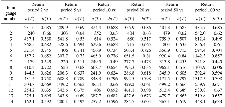
The Montana model, which predicts maximum rainfall in-tensity over duration t for the return period T as a power function of the duration (Eq. 1) (Burlando and Rosso, 1996), was adopted by DGRE-ST2i (2007). The estimated model parametersa(T )andb(T )are reported.

I (t, T )=a (T )∗t−b(T ), (1)

whereT is the return period (in years). Here, we adopt the hydrological risk definition where the risk isp=1/T (Bobée and Ashkar, 1993) so that we may consider thatT reflects the hydrological risk,tis rainfall duration in minutes, anda(T )

andb(T )are Montana IDF model parameters.

2.3 Geostatistical framework for IDF parameters

In this studya(T )andb(T )are taken as geostatistical vari-ables (Matheron, 1965). In fact, it is assumed that it is possi-ble to represent thea(T )andb(T )spatial structures through variogram functions. Furthermore, the analysis is made pos-sible by the fact that the two parametersa(T )andb(T )are known at the same experimental points.

Further, we first test whethera(T )andb(T )are dependent or independent. For this, their experimental cross-variogram

γa(T )b(T ) (Chilès and Delfiner, 1999) is examined (Eq. 2).

The experimental cross-variogram is defined as the variance of the difference between two variables of different types or attributes at two locations.

γa(T )b(T )(h)=

1

2∗N (h)

N (h) X

i=1

[a (xi+h)−a (xi)]

[b (xi+h)−b(xi)]

, (2)

whereN (h) represents the number of sample points sepa-rated by interdistanceh, andxiandxi+hare sampling

loca-tions separated by interdistanceh.

For the cross-correlation analysis, it is recommended to adopt the co-dispersion coefficient graphra(T )b(T )(h)

(Math-eron, 1965), which is linked to the cross-variogram and to the

direct variograms by

ra(T )b(T )(h)=γa(T )b(T )(h)

._p

γa(T )a(T )(h)∗γb(T )b(T )(h)

, (3)

whereγa(T )a(T ) andγb(T )b(T ) are the direct variograms

re-spectively ofa(T )andb(T ).

Generally, the direct variogram function is a key tool to quantify the variability associated with the regionalized vari-able,Z(the variableZ is set asa(T )orb(T )). The experi-mental semivariogram,γ (h), is calculated from the data as a function of the point separation,h,and is given by

γ (h)= 1

2N (h)

N (h) X

i=1

[Z(xi+h)−Z(xi)]2, (4)

whereN (h)is the number of sample points separated byh,

xi andxi+hare sampling locations separated by a distance

h, andZ(xi)andZ(xi+h)are values of the variableZ

mea-sured at the corresponding locations.

The sample variogram is fitted to a variogram model. For a stationary regionalized variable, the variogram is charac-terized by three main parameters: range, sill, and nugget. “Range” is the distance at which measurements cease to be correlated with each other. “Sill” is the variogram value at and beyond the range distance. The “nugget” effect is the ran-dom component of the digital values, graphically expressed by the discontinuity of the variogram at the origin. A para-metric approach is used to derive the variogram model. With-out loss of generality, further developments are given for the example of the spherical model in Eq. (5), which is a bounded variogram:

γδ(h)=s (δ)∗

h

1.5∗ hr (δ)−0.5∗ hr (δ)3i. (5)

The sills(δ)represents the highest variance for a large data point distance, and, for the spherical model, the ranger(δ)

refers to the distance over which the data are correlated. The crossed and direct variograms are estimated from the pairs (a(T ),b(T )) estimated at each observed location for the various durations (t=5, 10, 15, 20, 30, 45, 60, 120 and 180 min).

It is assumed that if the graphra(T )b(T )(h) is constant, it

may be concluded that the parametersa(T )andb(T )are de-pendent (Chilès et al., 1991).

(4)

4262 A. Chebbi et al.: Development of a method of robust rain gauge network optimization 18 # # # # # # # # # # # # % [ %[ % [ %[ % [ % [ % [ % [ % [ % [ % [ % [ % [ $ T$T $T $ T $T $ T $T $T

$

T $T $T $T $T $

T $T $T $T $ T $T $T

$ T $T $

T $T $ T $

T $T $T $

T $T $T $T $

T $T $ T

$ T

$ T $T

$ T $ T $ T $

T $T

$ T $

T $

T $T $T $T $ T $ T $ T $ T $T $T

$ T $ T

$ T $T $ T BV 6 BV 5 BV 4 BV 3

0 6 0 0 0 0 1 2 0 0 0 0 K i l o m e t e r s

# 1 4 s t u d i e d s t a t i o n s f o r I D F

%

[ I n i t i a l n e t w o r k

$

T 6 0 c a n d i d a t e s t a t i o n s

Figure 1. Location of rain gauges in the study area (Medjerda basin BV5; Northern coast basins BV3 and surrounding basins Meliane Basin BV4; Central Tunisia basins BV6)

Mediterranean Sea

Algeria

Fig. 1. Location of rain gauges in the study area (Medjerda basin

BV 5; northern coast basin BV 3; and surrounding basins (Meliane basin BV 4 and central Tunisia basin BV 6)).

average (spatial mean over the study domain) kriging error of

a(T )is the specific approach proposed here. Six return

peri-ods (T =2, 5, 10, 20, 50, 100 yr) covering a broad panoply of risk situations are considered.

Asa(T )andb(T )are not independent, it is proposed to

develop the kriging estimate ofa(T ) using b(T ) as infor-mation. External drift kriging (EDK) is a suitable method to achieve this goal. In fact, in the case of a sparse network, kriging with external drift seems more appropriate than or-dinary kriging. EDK requires knowledge of the values of

b(T )at the locations wherea(T )is to be interpolated. This is

achieved by first using an ordinary kriging approach tob(T ).

Therefore, a map ofb(T ) is produced that is then adopted to interpolatea(T ). The kriging systems are set out in Ap-pendix A.

2.4 The objective function

[image:4.595.52.284.61.227.2]

The decision model presented here is built within the frame-work of robust optimization and is inspired by the case stud-ies reported in Mulvey et al. (1995). The objective func-tion is written using the concept of regret by considering a quadratic term expressing the difference, for each scenario, between the values of the standardized mean spatial kriging variance achieved by the solution to be implemented and by the optimal solution for the scenario. This means that the op-timal solution for the model proposed will be solution-robust (Laguna, 1998). As such, the optimal solution obtained will be “close” to the optimum for any of the realized scenarios ensuring the optimality robustness. The robust optimization method adopted requires knowledge of a time horizon. For a fixed hydrologic riskp=1/T, whereT is the return period, we express the probability of an overrun of the event of return periodT during time horizon of durationN. It corresponds

Table 1. Studied rain gauges by DGRE-ST2i (2007).

Rain Rain Time Begining

gauge gauge series of

name number Basin size recording

Ghardimaou 1 BV 5 26 yr 29 Dec 1973

Zouarine gare 2 BV 5 33 yr 30 Sep 1968

Aïn Taga 3 BV 5 32 yr 9 May 1964

Aïn Beya Fernana 4 BV 5 17 yr 1 Jan 1983

Haïdra Poste Douanes 5 BV 5 17 yr 5 Mar 1984

Izid Barrage 6 BV 5 10 yr 28 Jul 1973

Joumine Antra 7 BV 3 28 yr 21 Aug 1963

Mellègue K13 8 BV 5 17 yr 15 Dec 1976

Oued Tine cassis 9 BV 3 20 yr 12 Jul 1968

Sarrat Pont Route 10 BV 5 18 yr 21 Oct 1982

Sejnène 11 BV 3 15 yr 19 Sep 1962

Siliana Laouej 12 BV 5 14 yr 5 Feb 1974

Slouguia 13 BV 5 15 yr 3 Jan 1976

Sraya Ecole 14 BV 5 26 yr 16 Dec 1975

to

u(T )=1−(1−p)N, (6)

whereN is the number of years in the horizon. Two time horizons are successively considered in the present study: the short term (N=5 yr) and the long term (N=30 yr).

u(T )is further scaled by dividing it by the sum ofu(T )

over the various return periods.

ω(T )=u(T ).Xi=N T

i=1 u(Ti), (7)

whereN T is the number of return periods; this means the number of scenarios considered in the study.

To evaluate the mean spatial kriging error variance over the study domain, a grid mesh with a resolution of 4 km was used. The optimization problem consists of minimizing the objective function expressed by

Min

N T X

i=1

ω (T =Ti)∗(S (T =Ti)−Sref(T =Ti))2, (8)

where

N T P

i=1

ω (T =Ti)=1wit hω(T =Ti) as indicated in

(Eq. 7), withSref(T=Ti)being the value of the

standard-ized mean spatial kriging variance obtained for every return periodTiindependently of the other return periods. It is taken

as reference.

In addition, standardization of the mean spatial kriging variance is obtained by using the interquartile range ofa(T )

kriging error variance map:

S (T =Ti)=

n X

i=1

σi(a(T=Ti))

2.

n

!,

[image:4.595.307.548.80.267.2]

(5)

19

-1,50 -1,00 -0,50 0,00 0,50 1,00 1,50

0 50000 100000 150000 200000 250000

h (m)

r

a(

2 an

s

)b

(2

a

n

s)

Mean of ra(2 ans)b(2ans)

(a) case 1 : T= 2 years

0,00 0,20 0,40 0,60 0,80 1,00 1,20

0 50000 100000 150000 200000 250000

h (m)

r

a(5

an

s)

b

(5 a

n

s)

Mean of ra(5 ans)b(5 ans)

(b) case 2 : T= 5 years

-0,2 0 0,2 0,4 0,6 0,8 1 1,2

0 50000 100000 150000 200000 250000

h (m)

r

a(10

an

s)

b

(10 a

n

s

)

(c) case 3 : T= 10 years

-0,2 0 0,2 0,4 0,6 0,8 1 1,2

0 50000 100000 150000 200000 250000

h (m)

r

a(20

an

s)

b

(20 a

n

s

)

(d) case 4 : T= 20 years

-0,0002 -0,0001 0 0,0001 0,0002 0,0003 0,0004 0,0005 0,0006 0,0007

0 50000 100000 150000 200000 250000

h (m)

r

a(5

0

an

s)b

(50

an

s)

(f) case 6 : T= 100 years

-0,2 0 0,2 0,4 0,6 0,8 1 1,2

0 50000 100000 150000 200000 250000

h (m)

r

a(

50

a

n

s)

b

(50

a

n

s)

[image:5.595.312.484.59.467.2]

(e) case 5 : T= 50 years

[image:5.595.113.487.66.465.2]

Figure 2. Fluctuation of ra(T)b(T)(h)

Fig. 2. Fluctuation ofra(T )b(T )(h).

where (σ_i(a(T2 ₌_T

i)))is the variance of kriging errors ofa(T=

Ti)at the computing nodei depending on locations of

sta-tions, andnis the number of grid nodes.

F (T =Ti)=

σ_{75 %}2 _(a(T=T i))−σ25 %2 (a(T=T i))

(10)

σ_{75 %}2 _(a(T₌_T

i))is the 75th percentile of the pattern of the

vari-ance of kriging errors ofa(T =Ti).

σ_{25 %}2 _(a(T₌_T

i)) is the 25th percentile of the pattern of the

variance of kriging errors ofa(T =Ti).

This objective function is subjected to domain constraints expressed by the set of possible locations for the stations (as such the solution space is defined).

In all cases (for the two horizons with the four differ-ent scenarios of network augmdiffer-entation (+25 %; +50 %; +100 %; +160 %)), the minimization problem is solved using a simulated annealing algorithm (Kirkpatrick et al., 1983).

3 Case study and data

(6)

[image:6.595.79.514.82.288.2]

Table 2. Parametersa(T )andb(T )for the 14 stations studied for IDF (DGRE-ST2i, 2007).

Rain Return Return Return Return Return Return

gauge period 2 yr period 5 yr period 10 yr period 20 yr period 50 yr period 100 yr

number a(T ) b(T ) a(T ) b(T ) a(T ) b(T ) a(T ) b(T ) a(T ) b(T ) a(T ) b(T )

1 231.6 0.685 289.9 0.69 324.4 0.688 356.9 0.686 401.3 0.685 435.7 0.685

2 240 0.66 303 0.64 352 0.63 404 0.63 479 0.62 542.0 0.62

3 437.1 0.538 541.8 0.53 614 0.524 680 0.517 759.9 0.507 812.4 0.498

4 368.5 0.682 528.6 0.694 629.6 0.683 715 0.665 804 0.635 856.4 0.61

5 321.4 0.745 406 0.741 456.9 0.734 503.4 0.726 556.9 0.713 594.4 0.704

6 157.7 0.652 307.7 0.73 465.9 0.776 651.5 0.81 920.4 0.84 1142.3 0.857

7 179 0.549 220 0.511 249.5 0.49 277.7 0.473 313.8 0.455 341.8 0.445

8 410.4 0.722 553 0.68 668.7 0.654 793.3 0.635 965.1 0.616 1103.9 0.606

9 144.5 0.626 206.3 0.637 241.9 0.624 286.8 0.618 345.9 0.605 392.4 0.594

10 431.5 0.758 688.3 0.789 848.3 0.796 992.5 0.798 1171.5 0.797 1317.5 0.798

11 304.8 0.669 349.2 0.663 385.4 0.66 429.2 0.661 499.2 0.666 559.9 0.671

12 254.2 0.635 342.6 0.675 406 0.692 461.1 0.698 512.4 0.689 530.8 0.67

13 275.1 0.695 343.8 0.69 387.7 0.682 427.6 0.673 479.7 0.663 519.8 0.657

[image:6.595.77.256.349.461.2]

14 162.1 0.592 200.1 0.592 237.2 0.596 284.7 0.604 367.1 0.619 448.1 0,633

Table 3. Adjusted sills and ranges fora(T ) and b(T )assuming

spherical variogram models.

Return

period Range Range

T (yr) Sill b b (km) Sill a a (km)

2 0.004 30 15 000 40

5 0.008 40 32 000 50

10 0.010 40 45 000 45

20 0.014 40 50 000 50

50 0.016 40 110 000 50

100 0.018 40 110 000 50

3.1 Results

3.2 Dependence of the parametersa(T )andb(T )

The co-dispersion coefficient graphra(T )b(T )(h)is plotted in

Fig. 2. An erratic fluctuation ofra(T )b(T )(h) around a fixed

value can clearly be seen. Therefore,ra(T )b(T )(h)can be

as-sumed as nearly constant for allT values, allowing the sup-position that a(T ) andb(T )are dependent variables. This authorizes the kriging of a(T ) by taking b(T ) as external drift.

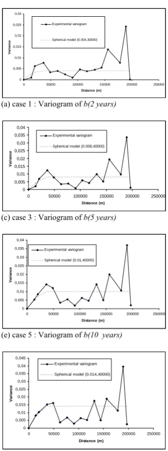
3.3 Structural analysis of the parametersa(T )andb(T )

Spherical variogram models are adjusted to sample vari-ograms. The ranges and sills were identified manually, and an attempt was made to take account of a good approxima-tion of the first points of the sample variograms (short in-terdistances) as well as a good approximation of high

inter-Table 4. Values ofu(T )andω(T ).

T (yr) Horizon= 5 yr Horizon= 30 yr

u(T ) ω(T ) u(T ) ω(T )

2 0.97 0.56 1 0.41

5 0.67 0.39 1 0.41

[image:6.595.312.545.465.541.2]

50 0.10 0.05 0.45 0.18

Table 5. Values of OF_ref(T )objective function obtained for

inter-polation ofa(T ).

Return period T 2 yr 5 yr 50 yr

25 % (scenario 1: 3 new stations) 2.13 1.69 1.67

50 % (scenario 2: 6 new stations) 1.52 1.34 1.35

100 % (scenario 3: 13 new stations) 1.30 1.05 1.06 Normative density of the WMO (160 %)

(scenario 4: 21 new stations) 1.03 0.89 0.89

distances. Table 3 reports the adjusted sill and range for ev-ery return period. Adjusted ranges ofa(T )andb(T )extend from 30 to 50 km. Sample and adjusted variograms ofa(T )

andb(T )are plotted in Fig. 3. Instead of using all the return

(7)

20

0 0,005 0,01 0,015 0,02 0,025 0,03

0 50000 100000 150000 200000 250000

Distance (m)

V

a

ri

ance

Experimental variogram

Spherical model (0.004,30000)

0 5000 10000 15000 20000 25000 30000 35000 40000

0 50000 100000 150000 200000 250000

Distance (m)

V

a

ri

an

ce

Spherical model (15000,40000)

(a) case 1 : Variogram of b(2 years) b) case 2 : Variogram of a(2 years)

0 0,005 0,01 0,015 0,02 0,025 0,03 0,035 0,04

0 50000 100000 150000 200000 250000

Distance (m)

Va

ri

a

n

c

e

0 20000 40000 60000 80000 100000 120000 140000

0 50000 100000 150000 200000 250000

Distance (m)

Va

ri

a

n

c

e

(c) case 3 : Variogram of b(5 years) d) case 4 : Variogram of a(5 years)

0 0,005 0,01 0,015 0,02 0,025 0,03 0,035 0,04

0 50000 100000 150000 200000 250000

Distance (m)

Va

ri

a

n

c

e

0 20000 40000 60000 80000 100000 120000 140000 160000 180000 200000

0 50000 100000 150000 200000 250000

Distance (m)

V

a

ri

an

ce

(e) case 5 : Variogram of b(10 years) f) case 6 : Variogram of a(10 years)

0 0,005 0,01 0,015 0,02 0,025 0,03 0,035 0,04 0,045

0 50000 100000 150000 200000 250000

Distance (m)

V

a

ri

an

ce

0 50000 100000 150000 200000 250000 300000

0 50000 100000 150000 200000 250000

Distance (m)

V

a

ri

an

ce

[image:7.595.113.284.57.515.2]

(g) case 7 : Variogram of b(20 years) h) case 8 : Variogram of a(20 years)

Fig. 3. Variograms ofa(T )andb(T ).

3.4 Comparison of the resulting robust networks

We first calculated the probability of overrun of the event

u(T )during the time horizon (Eq. 6) and thus the associated

weightω(T )(Eq. 7). Table 4 summarizes the values ofu(T )

andω(T )for each return period for the two horizons. In the

case of the short-term time horizon, we find thatT =50 yr is nearly neglected, and there is more focus onT =2 yr in the weighting system. For the long-term time horizon, the method assigns equal weights to normal and moderate risk (2 and 5 yr) while more weight is assumed for high risk sit-uations (T =50 yr). Therefore, these findings are consistent

with the intuitive point of view. Table 5 reports the values of the standardized variances OFref(T ), which obviously de-creased as the network size inde-creased (Table 5). It was also found that the most improvement is obtained when one splits from scenario 1 (three new stations to implement) to scenario 2 (six new stations to implement).

(8)

[image:8.595.53.543.81.152.2]

Table 6. Robust solutions. The locations which are different for the two horizons are in italics.

Increasing the existing network by horizon= 5 yr horizon= 30 yr

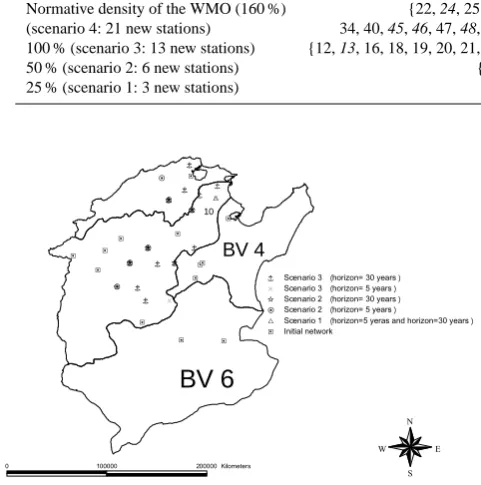
Normative density of the WMO (160 %) {22, 24, 25, 26, 27, 29, 30, 31, 32, {22, 25, 26, 27, 28, 29, 30, 31, 33, (scenario 4: 21 new stations) 34, 40, 45, 46, 47, 48, 49, 50, 51, 53, 54, 55} 34, 35, 36, 40, 47, 50, 51, 52, 53, 54, 58, 60} 100 % (scenario 3: 13 new stations) {12, 13, 16, 18, 19, 20, 21, 22, 25, 27, 28, 31, 35} {12, 16, 18, 19, 20, 21, 22, 25, 27, 31, 32, 35, 40)}

50 % (scenario 2: 6 new stations) {15, 18, 21, 25, 27, 34} {15, 18, 20, 21, 25, 27}

25 % (scenario 1: 3 new stations) { 25, 27, 28} { 25, 27, 28}

22 %

[ %[

% [ %[

% [

% [ % [

% [

% [ % [

$

T

$

T $T

#

Y

#

Y

#

Y

#

Y

#

Y

#

Y

Ú Ú Ú

N N N N N N

N N N N N

N N

Î Î Î Î Î

Î Î Î Î

Î Î Î

Î

BV 6

BV 4 10

0 1 0 0 0 0 0 2 0 0 0 0 0 K i l o m e t e r s

N

E W

S

% [ I n i t i a l n e t w o r k

$

T S c e n a r i o 1 ︵h o r i z o n = 5 y e r a s a n d h o r i z o n = 3 0 y e a r s ︶

#

Y S c e n a r i o 2 ︵h o r i z o n = 5 y e a r s ︶

Ú S c e n a r i o 2 ︵h o r i z o n = 3 0 y e a r s ︶

N S c e n a r i o 3 ︵h o r i z o n = 5 y e a r s ︶

Î S c e n a r i o 3 ︵h o r i z o n = 3 0 y e a r s ︶

Figure 4.Configuration of optimal networks

Fig. 4. Configuration of optimal networks.

are independent of the time horizon. This kind of network reinforcing is needed, without doubt. For scenario 2, which consists of adding six new stations chosen from 40 candi-dates, the two robust networks differ only by one station, for both time horizons. This also indicates good accuracy of the result. Five new stations can be added, and they are equally representative for the short- and long-term perspectives. For scenario 3, which requires 13 new locations to be found (out of 40 candidates), the two robust networks obtained in turn for the short- and long-term horizons differ only by 2 sta-tions. Hence, as many as 11 new locations are common to the two time horizon perspectives, which is a very encour-aging result from a decision making point of view. However, using 60 candidates for scenario 4, the short and long-term visions differ by 7 stations out of 21 (Fig. 4), which may be seen as problematic by a network manager.

In a previous paper (Chebbi et al., 2011), mono-objective criteria have been considered assuming 1 h rainfall intensity interpolation and erosivity factor interpolation and using one single extreme rainfall event to conduct the analysis. The comparison of previous results with the present study high-lights that the mean spatial kriging variance in the case of the mono-objective criterion is lower than or equal to that ob-tained in the case of the robust optimization. Nevertheless, the essential advantage of the robust optimization lies in the fact that it allows overcoming the problem of using one single rainfall event and yields networks which work “adequately”,

when considering various extreme events with different re-turn periods.

4 Conclusions

The robust optimization approaches are recommended in cases where the variables of interest are uncertain . The hydrological risk is considered in the present study, which aims to find new observation locations for rain gauges for recording short duration rainfall. The novel approach con-sists of considering IDF curve parameters to locate the best sites for installing imaginary new rain gauges. The method assumes a time horizon to minimize an objective function-based IDF parametera(T ) of the Montana model, consid-ering the weighting of various return periodsT. Kriging in-terpolation using the variance-reduction method was applied to build the objective function using the variance error of

a(T )estimation. The weighted mean spatial error variance

was considered.

[image:8.595.47.288.99.342.2]

(9)

Appendix A

Kriging systems

Once a proper variogram model is chosen, kriging is applied to the entire area of study to estimate the variable values at unsampled points, using the data from the surrounding sam-pled area. The kriging estimator is expressed as follows:

Z∗(x0)=

N X

i=1

λiZ(xi), (A1)

whereZ∗(x0)is an estimated value ofZ at locationx0,λi

is the weight assigned to the observation at the locationxi,

andNis the number of observations within the search neigh-bourhood.

Theλi’s are kriging weights which are estimated as the

solution of the ordinary kriging system (Eq. 2):



    

    

Nnb

P

i=1

λjγ (xj−xi)+µ

0

=γ (xj−x0)j=1, ...,Nnb

Nnb

P

i=1

λi=1

, (A2)

whereµ0 is a Lagrange parameter accounting for the con-straints on the weights.

The kriging variance for ordinary kriging is obtained by

σ₀2=γ (0)−

Nnb

X

i=1

λiγ (xi−x0)−µ

0

. (A3)

In the case of a sparse network, kriging with external drift seems more appropriate than ordinary kriging. Kriging with external drift represents the kriging estimates,Z∗(x), as a sum of a trend componentm(x)=E[Z(x)] and a residual

R(x)(Bardossy and Lehmann, 1998):

Z∗(x)=m(x)+R(x). (A4)

The trend component is then replaced by

E[Z(x)|Y (x)]=m(x)=a0+a1Y (x), (A5)

wherea0anda1are unknown constants. The linear estimator (Eq. 1) should be unbiased for anya0anda1values.

The external drift kriging variance is obtained by

σ₀2(x)=γ (0)−

N X

i=1

λiγ (xi−x)−µ1−µ2Y (x), (A6)

whereµ1andµ2 are two Lagrange parameters accounting for the constraints on the weights. Therefore,Y has to be known at locationsxi as well as at the target locationx0.

Acknowledgements. The data are taken from the Tunisian Water

Resources Department, DGRE (Tunisia). It is part of the Project “Modernisation et maintenance du réseau pluviométrique et pluviographique du Nord de la Tunisie”, which was financed by DGRE (2006). This work was partly supported by the scientific bilateral cooperation project between Tunisia and Portugal entitled “Modèles de gestion des bassins versants” (2005–2006).

Edited by: E. Gargouri-Ellouze

References

Afonso, P. and Cunha, M. C.: Robust optimal design of activated sludge bioreactors, J. Environ. Eng., 133, 44–52, 2007. Bai, D., Carpenter, T., and Mulvey, J.: Making a case for robust

optimization models, Manage. Sci., 43, 895–907, 1997. Barca, E., Passarella, G., and Uricchio, V.: Optimal extension of the

rain gauge monitoring network of the Apulian regional consor-tium for crop protection, Environ. monitor. Assess., 145, 375– 386, 2008.

Bardossy, A. and Lehmann, W.: Spatial distribution of soil moisture in a small catchment. Part 1: Geostatistical analysis, J. Hydrol. (Amsterdam), 206, 1–15, 1998.

Beyer, H.-G. and Sendhoff, B.: Robust optimization – a compre-hensive survey, Computer Methods in Applied Mechanics and Engineering, 196, 3190–3218, 2007.

Bobée, B. and Ashkar, F.: The gamma family and derived distribu-tions applied in hydrology, Water Resources Publicadistribu-tions, Little-ton, Colorado, 203 pp., 1991.

Bras, R. L. and Rodríguez-Iturbe, I.: Network design for the esti-mation of areal mean of rainfall events, Water Resour. Res., 12, 1185–1195, 1976.

Burlando, P. and Rosso, R.: Scaling and muitiscaling models of depth-duration-frequency curves for storm precipitation, J. Hy-drol., 187, 45–64, doi:10.1016/S0022-1694(96)03086-7, Frac-tals, scaling and nonlinear variability in hydrology, 1996. Chebbi, A., Kebaili Bargaoui, Z., and Da Conceiçao Cunha, M.:

Optimal extension of rain gauge monitoring network for rainfall intensity and erosivity index interpolation, J. Hydrol. Eng., 16, 665–676, 2011.

Chen, Y.-C., Wei, C., and Yeh, H.-C.: Rainfall network design using kriging and entropy, Hydrol. Process, 22, 340–346, 2008. Chilès, J. P. and Delfiner, P.: Geostatistics, Wiley Series in

Probabil-ity and Statistics: Applied ProbabilProbabil-ity and Statistics, John Wiley & Sons Inc., New York, doi:10.1002/780470316993, Modeling spatial uncertainty, A Wiley-Interscience Publication, 1999. Chilès, J. P., Gable, R., and Morin, R. H.: Contribution de la

géo-statistique à l’étude de la thermicité des rides océaniques du Paci-fique. Cahiers de Géostatistiques, Fascicule 1, Compte-rendu des Journées de Géostatistique, 6–7 Juni 1991, Fontainebleau, 51– 61, 1991.

Cunha, M. C. and Sousa, J. J. O.: Robust Design of Water Dis-tribution Networks for a Proactive Risk Management, J. Water Resour. Plng. and Mgmt., 136, 227–236, 2010.

Delhomme, J. P.: Kriging in the hydrosciences, Adv. Water Resour., 1, 51–266, 1978.

(10)

Hydraccess: IRD, available at: http://www.mpl.ird.fr/hybam/outils/ ha4_fr_dn.php (last access: 2007), 2000.

Kirkpatrick, S., Gelatt, C. D., and Vecchi, M. P.: Optimization by Simulated Annealing, Science, 220, 671–680, 1983.

Koutsoyiannis, D., Kozonis, D., and Manetas, A.: A mathematical framework for studying rainfall intensity-duration-frequency re-lationships, J. Hydrol., 206, 118–135, 1998.

Laguna, M.: Applying robust optimization to capacity expansion of one location in telecommunications with demand uncertainty, Manage. Sci., 44, S101–S110, 1998.

Matheron, G.: Les Variables régionalisées et leur estimation, Mas-son, Paris, 305 pp., 1965.

Moss, M. E. and Tasker, G. D.: An intercomparison of hydrological network-design technologies, Hydrol. Sci. J., 36, 209–221, 1991. Mulvey, J. M., Vanderbei, R. J., and Zenios, S. A.: Robust optimiza-tion of large-scale systems, Operaoptimiza-tions Res., 43, 264–281, 1995. Pardo-Iguzquiza, E.: Optimal selection of number and location of rainfall gauges for areal rainfall estimation using geostatistics and Simulated Annealing, J. Hydrol., 210, 206–220, 1998.

Ricciardi, K. L., Pinder, G. F., and Karatzas, G. P.: Efficient ground-water remediation system design subject to uncertainty using ro-bust optimization, J. Water Resour. Plan. Manage., 133, 253–263, 2007.

Watkins, D. W. and McKinney, D. C.: Finding robust solutions to water resources problems, J. Water Resour. Plan. Manage., 123, 49–58, 1997.

World Meteorological Organization (WMO): Guide to hydrologi-cal practices, Data acquisition and processing, analysis forecast-ing and other applications, Design and evaluation of hydrological networks, WMO, 168, Geneva, Switzerland, 1994.