Hydrol. Earth Syst. Sci., 17, 1161–1175, 2013 www.hydrol-earth-syst-sci.net/17/1161/2013/ doi:10.5194/hess-17-1161-2013
© Author(s) 2013. CC Attribution 3.0 License.
EGU Journal Logos (RGB)
Advances in
Geosciences
Open Access
Natural Hazards
and Earth System
Sciences
Open AccessAnnales
Geophysicae
Open AccessNonlinear Processes
in Geophysics
Open AccessAtmospheric
Chemistry
and Physics
Open AccessAtmospheric
Chemistry
and Physics
Open Access DiscussionsAtmospheric
Measurement
Techniques
Open AccessAtmospheric
Measurement
Techniques
Open Access DiscussionsBiogeosciences
Open Access Open Access
Biogeosciences
DiscussionsClimate
of the Past
Open Access Open Access
Climate
of the Past
Discussions
Earth System
Dynamics
Open Access Open Access
Earth System
Dynamics
DiscussionsGeoscientific
Instrumentation
Methods and
Data Systems
Open Access
Geoscientific
Instrumentation
Methods and
Data Systems
Open Access DiscussionsGeoscientific
Model Development
Open Access Open Access
Geoscientific
Model Development
DiscussionsHydrology and
Earth System
Sciences
Open AccessHydrology and
Earth System
Sciences
Open Access DiscussionsOcean Science
Open Access Open Access
Ocean Science
DiscussionsSolid Earth
Open Access Open Access
Solid Earth
DiscussionsThe Cryosphere
Open Access Open Access
The Cryosphere
DiscussionsNatural Hazards
and Earth System
Sciences
Open Access
Discussions
GloFAS – global ensemble streamflow forecasting and flood
early warning
L. Alfieri1,2, P. Burek2, E. Dutra1, B. Krzeminski1, D. Muraro2, J. Thielen2, and F. Pappenberger1,3 1European Centre for Medium-Range Weather Forecasts, Reading, UK
2European Commission – Joint Research Centre, Institute for Environment and Sustainability, Ispra, Italy 3College of Hydrology and Water Resources, Hohai University, Nanjing, China
Correspondence to: L. Alfieri ([email protected])
Received: 15 October 2012 – Published in Hydrol. Earth Syst. Sci. Discuss.: 2 November 2012 Revised: 27 February 2013 – Accepted: 28 February 2013 – Published: 15 March 2013
Abstract. Anticipation and preparedness for large-scale flood events have a key role in mitigating their impact and op-timizing the strategic planning of water resources. Although several developed countries have well-established systems for river monitoring and flood early warning, figures of pop-ulations affected every year by floods in developing coun-tries are unsettling. This paper presents the Global Flood Awareness System (GloFAS), which has been set up to pro-vide an overview on upcoming floods in large world river basins. GloFAS is based on distributed hydrological simula-tion of numerical ensemble weather predicsimula-tions with global coverage. Streamflow forecasts are compared statistically to climatological simulations to detect probabilistic exceedance of warning thresholds. In this article, the system setup is de-scribed, together with an evaluation of its performance over a two-year test period and a qualitative analysis of a case study for the Pakistan flood, in summer 2010. It is shown that hazardous events in large river basins can be skilfully detected with a forecast horizon of up to 1 month. In ad-dition, results suggest that an accurate simulation of initial model conditions and an improved parameterization of the hydrological model are key components to reproduce accu-rately the streamflow variability in the many different runoff regimes of the earth.
1 Introduction
Weather-driven natural hazards, including storm surges, floods, flash floods, and subsequent mass movements, are the most prominent natural disasters in worldwide statistics
(CRED, 2011). A total of 57 % of the reported number of vic-tims in 2011 are associated with so-called “hydrological dis-asters”. These have caused a total economic damage of more than 70 billion US dollars, meaning a 230 % average increase compared to the previous decade (Guha-Sapir et al., 2012). According to the United Nations International Strategy for Disaster Reduction (UN/ISDR, 2002) and statistics from surance companies, the socioeconomic impact of floods is in-creasing. With steadily rising world population, the need for optimizing the use of water resources for drinking water as well as energy production demands more and more techno-logically driven solutions for controlling water quantity and quality in river systems. In addition, floods can no longer be treated as isolated events, as they are heavily linked with is-sues such as food insecurity, disease outbreaks and environ-mental degradation (IFRC, 2011).
natural disasters, the European Union Solidarity Fund (Euro-pean Commission, 2002) being the main example for Europe, developing countries often struggle through a much longer recovery process. Increasing preparedness can be achieved by flood hazard maps, which are available on national or re-gional level (e.g., Hagen and Lu, 2011; Prinos et al., 2008) as well as on global level (Pappenberger et al., 2012; Winsemius et al., 2012). These static maps can be used to define flood hazard zones, but they do not incorporate changes in daily conditions, which require a real-time observing system.
The availability of remote sensing data, such as satellite imagery, has fostered the development of flood detection techniques at global scale (e.g., de Groeve, 2010; Proud et al., 2011; Westerhoff et al., 2013; Wu et al., 2012a), which promptly produce overviews of affected areas and improve the management of rescue actions. To increase the prepared-ness towards floods and in general to water-related haz-ards, a number of research institutes and national hydro-meteorological services run operational flood forecasting systems, often focused on specific river basins or, most com-monly, limited to national boundaries (Alfieri et al., 2012a). Several flood forecasting systems are based on observed river level, while future values are extrapolated through river rout-ing models or by couplrout-ing observed rainfall fields into hy-drological models. The extension of the forecast horizon be-yond the response time of a river basin is enabled by the use of numerical weather predictions (NWPs) as input to hydrological–hydraulic models (e.g., He et al., 2010; Hopson and Webster, 2010; Paiva et al., 2012; Thiemig et al., 2010). Recent review articles by Cloke and Pappenberger (2009) and by Alfieri et al. (2012a) showed the strong potential of using ensemble NWPs to further extend the forecasting hori-zon in early warning systems.
Weather forecasting models are set up at global scale in different meteorological centers, producing deterministic and ensemble products. Nevertheless, only few attempts have been made so far to move towards operational systems with coupled hydro-meteorological models producing streamflow predictions at the global scale (see Sperna Weiland et al., 2010; Voisin et al., 2011; Wang et al., 2011; Candogan Yossef et al., 2012) and, to the authors’ knowledge, none of these runs operationally with ensemble predictions. Indeed real-time hydrological modeling requires a large amount of information, including not only static maps describing the surface and sub-surface basin features, but also data assimila-tion techniques or a long-term balance of water fluxes to give an estimate of the initial conditions, from which the forecast is run. At the continental scale, the European Flood Aware-ness System (EFAS) has demonstrated that ensemble flood forecasting and early warning based on critical flood thresh-olds can be produced also with limited amount of data, by applying probabilistic methods and model consistent clima-tologies (Bartholmes et al., 2009; Pappenberger et al., 2010b; de Roo et al., 2003; Thielen et al., 2009a).
The aim of this study is to assess the feasibility of an en-semble flood forecasting and early warning system at the global scale, built up with a similar framework as that of EFAS, and to evaluate the system performance in its ini-tial stage, where no model parameter has been specifically calibrated. The Global Flood Awareness System (GloFAS) has been set up jointly between the Joint Research Centre (JRC) of the European Commission and the European Centre for Medium-Range Weather Forecasts (ECMWF), and has been running operationally on a daily basis since July 2011. GloFAS produces global flood forecasting products, which are shown on a password-protected web interface. The sys-tem performance is currently being monitored, and results are already being accessed for research and testing purposes by partner organizations such as the Mekong River Com-mission (http://www.mrcmekong.org/) and the CEMADEN (http://www.cemaden.gov.br/), the newly established Brazil-ian center for monitoring of natural disasters.
2 Data and methods
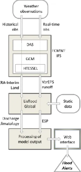
The GloFAS system is composed of an integrated hydro-meteorological forecasting chain and of a monitoring system that analyzes daily results and shows forecast flood events on a dedicated web platform. An overview of the system struc-ture is shown in Fig. 1.
2.1 Meteorological data
To set up a forecasting and warning system that runs on a daily basis with global coverage, initial conditions and input forcing data must be provided seamlessly to every point within the domain. To this end, two products are used. The first consists of operational ensemble forecasts of near-surface meteorological parameters. The second is a long-term dataset consistent with daily forecasts, used to derive a reference climatology. These products are described in the next sub-sections. They are both computed by the Integrated Forecast System (IFS) of the ECMWF, whose main compo-nents (see Fig. 1) are a data assimilation system (DAS) and a global circulation model (GCM).
2.1.1 Daily forecasts
Fig. 1. Overview of the GloFAS structure.
the land surface module (HTESSEL; see Sect. 2.2.1) of the IFS, which in turn creates the VarEPS runoff fields for the ensemble streamflow prediction.
2.1.2 Reference climatology
The second meteorological product used is ERA-Interim (Dee et al., 2011), the latest global atmospheric reanalysis produced by the ECMWF. The ERA-Interim archive con-tains 6-hourly gridded estimates of three-dimensional (3-D) meteorological variables, 3-hourly estimates of a large num-ber of surface parameters and other two-dimensional (2-D) fields. It has horizontal resolution of about 80 km, it cov-ers the period from 1 January 1979 onwards, and contin-ues to be extended forward in near-real time. ERA-Interim makes use of a forecast model, so that information can be ex-trapolated from locally observed weather parameters to un-observed parameters in a physically meaningful way. ERA-Interim precipitation dataset has been bias-corrected using the Global Precipitation Climatology Project (GPCP) version 2.1 (Huffman et al., 2009). The bias correction assumes a scale-selective rescaling that corrects ERA-Interim 3-hourly precipitation in order to match the monthly accumulation provided by GPCP at grid-point scale. The rescaling factor is obtained by the following: (i) interpolating conservatively GPCP at 2.5◦×2.5◦to the equivalent T95 Gaussian grid; (ii)
interpolating conservatively ERA-Interim from T255 Gaus-sian grid to T95 GausGaus-sian grid; (iii) computing the rescal-ing factor at the T95 resolution (observations resolution); and (iv) interpolating bi-linearly the rescaling factor from T95 to T255. This procedure has the advantage of preserving small-scale features of ERA-Interim (for instance related to oro-graphic effects) and correcting for large-scale bias.
2.2 Hydrological modeling
River discharge is simulated by the Lisflood hydrological model (van der Knijff et al., 2010) for the flow routing in the river network and the groundwater mass balance. The model is set up on global coverage with horizontal grid reso-lution of 0.1◦(about 10 km in mid-latitude regions) and daily time step for input/output data. Details of Lisflood and the HTESSEL are given in the following sections. Two types of simulations are performed to estimate discharge in the river network, which use the input runoff forcing described in the previous section and appropriate initial model state.
– Forecasting simulations are run every day using the lat-est VarEPS runoff prediction and result in 51 possible evolutions of the streamflow for the selected forecast horizon (i.e., 45 days in the current setting).
– A deterministic climatological simulation is run in of-fline mode using ERA-Interim/Land input data for a 21 yr period starting in 1990. Seamless streamflow cli-matology is derived, and maps of daily annual maxima are extracted and fitted with a Gumbel extreme value distribution to estimate corresponding discharge warn-ing thresholds for selected return periods.
2.2.1 HTESSEL
HTESSEL (Balsamo et al., 2009, 2011a) is the land sur-face component of the ECMWF IFS. It is a revised land surface Hydrology, derived from the former Tiled ECMWF Scheme for Surface Exchange over Land (TESSEL). HT-ESSEL computes the land surface response to atmospheric forcing, and estimates the surface water and energy fluxes and the temporal evolution of soil temperature, moisture con-tent and snowpack conditions. At the interface to the atmo-sphere, each grid box is divided into fractions (tiles), with up to six fractions over land (bare ground, low and high vege-tation, intercepted water, shaded and exposed snow). Vege-tation types and cover fractions are derived from an external climate database, based on the global land cover characteris-tic (Loveland et al., 2000).
law of diffusion, modified to take into account soil water freezing/melting. Water movement in the soil is determined by Darcy’s law, and surface runoff accounts for the subgrid variability of orography. In the case of a partially (or fully) frozen soil, water transport is limited, leading to a redirection of most of the rainfall and snowmelt to surface runoff when the uppermost soil layer is frozen. The snow scheme (Dutra et al., 2010) represents an additional layer on top of the soil, with an independent prognostic thermal and mass content. The model has been successfully tested in river routing set-tings (Balsamo et al., 2011b; Pappenberger et al., 2010a). HTESSEL is part of the IFS at ECMWF with operational ap-plications ranging from the short-range to monthly and sea-sonal weather forecasts.
For this work, operational ensemble forecasts of surface and sub-surface runoff (soil to groundwater percolation) are extracted from the daily output of the ECMWF forecasts and then resampled to 0.1◦resolution to be used as input by Lis-flood. These are produced by the HTESSEL module of the IFS using VarEPS weather forecasts as input. Further, an of-fline simulation of HTESSEL forced by ERA-Interim near-surface fields and bias-corrected ERA-Interim precipitation was performed to derive a 21 yr climatology starting in 1990, including surface and sub-surface runoff (hereafter referred to as ERA-Interim/Land).
Balsamo et al. (2012) presented a detailed description of the simulation setup of ERA-Interim/Land and a general overview of the model performance. In particular, the sim-ulated discharge (monthly means) improved in most conti-nents from using the surface and sub-surface runoff of ERA-Interim to the new fields produced by ERA-ERA-Interim/Land, as done in this study.
2.2.2 Lisflood global
Lisflood is a GIS-based spatially distributed hydrological model, which includes a one-dimensional channel routing model (van der Knijff et al., 2010). The Lisflood model is currently running within the European Flood Awareness Sys-tem (EFAS) on an operational basis (Pappenberger et al., 2010b; Thielen et al., 2009a) covering the whole of Europe on a 5 km grid.
In the context of global flood modeling, the transformation from precipitation to surface and sub-surface runoff is done by the HTESSEL module of the IFS, which accounts for ver-tical water fluxes and water/snow storage on a pixel basis. However, HTESSEL is not capable of simulating horizontal water fluxes along the river network. For this purpose, Lis-flood global is set up to simulate the groundwater and routing processes, using surface runoff and sub-surface runoff from HTESSEL as input fluxes on a resolution of 0.1◦. Surface runoff is routed via overland flow to the outlet of each cell using a four-point implicit finite-difference solution of the kinematic wave equations (Chow et al., 1988). The global land cover characteristic is used to assign Manning’s surface
roughness based on the cover class. Subsurface storage and transport are modeled using two linear reservoirs. The upper zone represents a quick runoff component, which includes fast groundwater and subsurface flow through macropores in the soil. The lower zone is fed by percolation from the upper zone and represents the slow groundwater component that generates the baseflow. Amount and timing of the outflow from the respective groundwater reservoirs to the outlet of each grid cell are controlled by two parameters that reflect the residence time of water in the upper and lower ground-water zone. Runoff produced for every grid cell from sur-face, upper and lower groundwater zones is routed through the river network using the same kinematic wave approach as for the overland flow. The river network is taken from the HydroSHEDS project (Lehner et al., 2008) and upscaled to 0.1◦by using the approach of Fekete et al. (2001). In the next developments the upscaled 0.1◦dataset of Wu et al. (2012b) will be used. River parameters like channel gradient, Man-ning’s coefficient, river length, width and depth were esti-mated from the digital elevation model, the river network and the upstream area. Further details of the Lisflood model can be found in van der Knijff et al. (2010). Within EFAS the parameters to control percolation to the lower groundwater zone, the residence time of the upper and lower zone and the routing parameter (a multiplier to Manning’s roughness) are calibrated using observed discharge time series (see Feyen et al., 2007). In the current setup of GloFAS, these parameters are set following typical ranges observed in EFAS-calibrated river basins, while their estimation through specific calibra-tion will be part of future works. In arid and semiarid re-gions, one can observe a loss of water among the channel reaches. In order to include this effect into the model, we use the simplified approach by Rao and Maurer (1996) to simulate transmission losses in a stream. This method uses a power function with two parameters to describe the rela-tionship between inflow and outflow in cells. In a first at-tempt the yearly average potential evapotranspiration rate is used to fit the transmission loss function. The resulting loss function gives emphasis to transmission losses in Africa, the Arabian Peninsula, India, Australia and the southern part of North America, whereas discharge in Europe and the north-ern part of Asia remains unaffected. With this approach the model is able to mimic the river–aquifer and river–floodplain interaction (e.g., the Sudd, the vast swamps in South Sudan along the Nile River) as well as the influence of evaporation from big braided rivers.
2.3 Operational forecasting
basins, with time of concentration of the order of one month. From day 16 to day 45, input maps of surface and subsur-face runoff are set to zero; therefore, the hydrological model (i.e., Lisflood) will simply convey towards the outlet water al-ready within each river basin. Initial condition maps to start up the model are first taken from the last available day of ERA-Interim dataset. Initial conditions for subsequent sim-ulations are then extracted from the results of the model run with the VarEPS control run, after the first day of simula-tion. As this procedure is based on forecast meteorological variables as input, rather than observed, results may possi-bly drift in time from reality. This could lead to biased ini-tial conditions and consequently to under- or over-estimating streamflow values, even where weather forecasts are accu-rate. Therefore, periodical updating of initial condition maps based on ERA-Interim dataset is foreseen for future system developments.
Resulting ESP maps for each daily time step and ensemble member are compared with reference threshold maps derived from the streamflow climatology, corresponding to return pe-riods of 2, 5 and 20 yr. Summary threshold exceedance maps are calculated accordingly, which show the maximum prob-ability of exceeding the 5 and 20 yr return period within the forecast horizon. In addition, reporting points are chosen at fixed and dynamic locations in the river network where up-coming flood hazard is detected, according to the following two-step procedure.
Fixed points are first selected from about 4000 gauged river stations included in the Global Runoff Data Centre (GRDC, http://grdc.bafg.de/) database, where the maximum daily forecast value of the ESP mean, over the simulation horizon, is above the 2 yr return period threshold.
Dynamic points are then generated to provide similar in-formation in river reaches where no fixed point is available. The following experience-based rules are adopted for obtain-ing a good overview of the potentially affected areas, yet avoiding the confusion of displaying too many points:
– The ESP mean is above the medium warning thresh-old on at least 5 contiguous pixels of the river network (∼50 km long river reach), in at least one of the two most recent daily simulations.
– The upstream area of the selected point must be larger than 4000 km2.
– Points are generated starting from the most downstream pixel complying with the selection criteria, proceeding upstream every 300 km to each other, unless a fixed point is encountered within a shorter distance.
The two sets of points are merged and classified into medium, high and severe alert level. Medium alert level (yellow color coding) is assigned to points with ESP mean between 2 and 5 yr return period. High alert level (red color coding) is as-signed to points with ESP mean between 5 and 20 yr return
period. Severe alert level (purple color coding) is assigned to points with ESP mean above 20 yr return period. At each point, ESP time series are plotted versus the forecast hori-zon, together with persistence diagrams (Bartholmes et al., 2009) showing the probability of exceeding the three warn-ing thresholds for each day of simulation and the evolution over the latest consecutive forecasts.
3 Performance evaluation
3.1 Evaluation of the hydrological modeling
The first part of the work is focused on evaluating the skill of the Lisflood hydrological model forced by ERA-Interim/Land runoff in reproducing the hydrological pro-cesses for river basins in different regions and climates of the earth. The 21 yr simulated discharge climatology has been compared with daily observations at a number of stations in-cluded in the GRDC database. Stations for the comparison were chosen according to the three following criteria:
– Observed discharge time series at each station must in-clude at least 5 yr of valid data within the simulation period (1990–2010).
– At each river station, the upstream area of the mod-eled river network must not differ by more than 10 % from the actual one, to prevent matching incoherent data pairs. This typically occurs in small river basins, where the modeled river network is sometimes different from the real one – because of scaling issues – and as a result the station does not lie in the correct grid cell.
– A visual check has been performed on the observed time series to remove those stations with evident dis-charge regulation (e.g., through artificial reservoirs) or with clear errors in the data.
Fig. 2. Coefficient of variation of the estimation residuals for the 620 stations considered. Circle size is proportional to the upstream area of the river station.
´
Obidos – linigrafo (Brazil), in the Amazon River, are com-pared over 17 yr between 1990 and 2007. The performance of simulation is assessed for each station through different skill scores: the Nash–Sutcliffe efficiency (NS), Pearson cor-relation coefficient (PCC), root mean square error (RMSE), mean absolute error (MAE) and coefficient of variation (CV) of the residuals towards the observed mean.
It is worth noting that the proposed system is designed for early warning purposes, rather than for quantitative stream-flow forecasting. In other words, the main goal of the system is to assign each forecast value a correct probability of occur-rence taken from its cumulative distribution function and thus identify extreme values in the upper tail of the distribution, which can possibly correspond to flooding conditions. Ide-ally, the percentile rank of each simulated value, compared to its climatology, should match that of observations (related to the observed time series), independently of any bias be-tween observed and simulated time series. As a result, more emphasis is given to skill scores that are not affected by bias of estimation. Also, dimensionless indicators are preferred, as these enable straightforward comparison of results from different river stations having a wide range of quantitative runoff and hydrological regimes. Among such skill scores, the coefficient of variation (CV) at each point is calculated as the ratio of the standard deviation (σ (.))of the estimation residuals to the mean (Qobs)of observations,
CV=σ (Qsim−Qobs)
Qobs (1)
The CV enables the comparison of the estimation variabil-ity at different locations through normalization by the aver-age flow conditions. Furthermore, the Pearson correlation co-efficient (PCC) of simulated versus observed discharges is calculated according to the following equation:
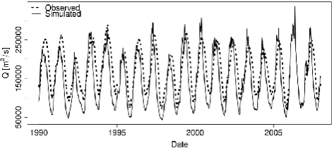
Fig. 3. Comparison between observed and simulated daily average discharge in the Amazon River at ´Obidos, linigrafo, Brazil.
PCC=
P
∀i Qobsi−Qobs
Qsimi−Qsim q
P
∀i Qobsi−Qobs
2qP
∀i Qsimi−Qsim
2, (2) which considers all thei-th available daily data pairs. PCC is particularly fit to the desired verification strategy as it as-sesses the linear correlation between simulated and observed discharges, without being penalized by multiplicative or ad-ditive bias. On the other hand the PCC is known for being sensitive to even a few outlying data pairs, thus stressing sig-nificant shifts between the timing of simulated and observed flow peaks (Wilks, 2006).
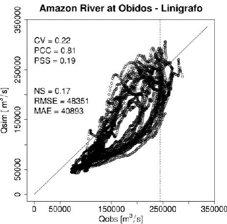
[image:6.595.310.547.294.399.2]Fig. 4. Scatter plot of observed and simulated daily average dis-charge (1990–2007) in the Amazon River at ´Obidos, linigrafo, Brazil. 90th percentiles used for threshold exceedance analysis are shown with dashed lines while skill scores are shown on the left side.
variables calculated from the set of observations and of sim-ulated values:
– hit: event observed and simulated;
– miss: event observed and not simulated;
– false alarm: event simulated and not observed;
– correct negative: event not observed and not simulated.
Peirce’s skill score (PSS, Eq. 3) (Hanssen and Kuipers, 1965) has been calculated for each station, taking the 90th per-centile as threshold values (i.e., the 90th perper-centile from the sorted observations and from the sorted simulated values to discriminate each corresponding data series).
PSS= hits hits+misses−
false alarms
false alarms+correct negatives (3) Such a percentile is a good tradeoff between being represen-tative of high flow values and including a sufficient number of events to draw robust statistics. Data series for comparison include at least five years of data, which corresponds to more than 182 days above the 90 % threshold. The PSS accounts for all elements of the contingency table and is defined as the difference between probability of detection (POD) and probability of false detection (POFD), PSS = POD−POFD. Perfect forecasts have PSS = 1, while forecasts have no skill when PSS≤0.
3.2 Performance of the early warning system
The early warning system, as described in Sect. 2.3, has been set up and has been running operationally since July 2011. To evaluate the forecast performance, the system was run in hindcast mode for the period 1 January 2009 to 31 Decem-ber 2010. A total of 730 sets (i.e., one per day) of 45-day en-semble streamflow predictions (ESPs) were evaluated against discharge proxy simulations for the same period, taken from the simulated discharge climatology obtained using ERA-Interim/Land runoff as forcing. Differently from the analy-sis in the previous section, this approach enables the perfor-mance evaluation at each grid point of the simulated river network. Comparison of streamflow forecasts with point ob-servations was not performed at this stage, due to insuffi-cient data availability for the selected period. Furthermore, as the datasets of streamflow predictions and proxy simu-lations are generated by the same hydrological model, this type of analysis focuses more on the skills of the ensemble weather predictions. Indeed, it allows one to draw indica-tions on the maximum forecast horizon (or potential skill) for which the system yields valuable information. In general, we expect results to be mainly influenced by (i) the skills of 15-day weather predictions and by (ii) the upstream area of each selected river point, which is correlated with the lag time be-tween rainfall events and the subsequent flow hydrographs. This can yield an extension of the forecast lead time beyond the time window for which weather forecasts are available and contribute to the assessment of the limits of predictabil-ity (Thielen et al., 2009b).
a flood forecasting system. A similar approach has been ap-plied in this work.
Ensemble streamflow predictions were evaluated by means of a twofold approach. The continuous rank probabil-ity skill score (CRPSS; e.g., Hersbach, 2000; Voisin et al., 2010) is used to evaluate the quantitative skills of predic-tion, while the area under the receiver operating character-istic (AROC; see Marzban, 2004; Wilks, 2006) is calculated to assess the performance in threshold exceedance analysis.
The CRPSS is defined as
CRPSS=CRPSref−CRPSforecast CRPSref
(4)
where
CRPS= ∞ Z
−∞
[F (y)−F0(y)]2dy (5)
and F0(y)=
0, y <observed value
1, y≥observed value (6)
while F (y) is the stepwise cumulative distribution func-tion (cdf) of the ESP for each forecast day and lead time. The CRPS accounts for the integrated squared difference between the ESP and the step function of the proxy truth (Wilks, 2006), here represented by the corrected climato-logical run for the 2 yr of forecast. The CRPSS is a dimen-sionless indicator of the skills of ensemble predictions, mea-sured by CRPSforecast, compared to that of a reference fore-cast CRPSref, which assumes all future values being equal to the latest observation (persistence criterion), meaning the value at timestepi=0 that is used to initialize each forecast. CRPSS ranges between 1 (for perfect predictions) and−∞, though ESPs are only valuable when CRPSS>0, i.e., when ensemble forecasts perform better than the reference persis-tent forecast.
[image:8.595.297.547.63.248.2]Receiver operating characteristic (ROC) curves are widely used to measure the skill of dichotomous forecasts based on probabilistic information, as they plot the empirical re-lation between the hit rate (HR) and false alarm rate (FAR) for different probability thresholds (Alfieri et al., 2012b). The overall performance of ensemble forecasts in predict-ing threshold exceedances can be assessed though the area under the ROC curve, which summarizes the system skill for all the probability thresholds, which in the discrete case are as many as the ensemble size. AROC values range between 0 (i.e., forecasts are exactly the opposite of observations) and 1 (perfect match between predicted and observed threshold exceedances). AROC = 0.5 corresponds to random forecasts, while meteorological ensemble predictions are commonly considered as useful when AROC≥0.7 (e.g., Buizza et al., 1999).
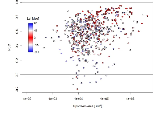
Fig. 5. Pearson correlation coefficient of simulated versus observed discharge for the 620 stations considered plotted against the cor-responding upstream area. Circle color depends on the latitude of each river station.
4 Results
4.1 Evaluation of the hydrological modeling
[image:8.595.45.182.191.338.2]Fig. 6. Peirce’s skill score of simulated versus observed discharge for the 620 stations considered. Circle size is proportional to the upstream area of the river station. The black-contoured rectangle indicates the area shown in Fig. 10.
points), where time series at these stations (not shown) sug-gest discrepancies to be related to the modeling of freezing cycles, snow accumulation and melting processes (modeled by HTESSEL), and the subsequent lag between simulated and observed peak discharge during spring.
In Fig. 5 the PCC is plotted against the upstream area of each gauge. In addition the gauge latitude is shown with a color shading ranging from red at the Equator, to blue at high latitudes. Figure 5 shows a tendency of higher correlations in large river basins (i.e., upstream area larger than 10 000 km2) in inter-tropical latitudes. Overall, 71 % of points have PCC larger than 0.5. The envelope curve of highest PCC values shows an increasing trend with the upstream area. In fact, the typical scales of weather events inducing floods in small river basins are below the spatial and temporal resolution of the hydrological model and of the meteorological input data used in simulation, as well as of the observations used for validation.
Peirce’s skill score (PSS) for the set of selected stations is shown in Fig. 6. A total of 98.5 % of stations provide skill-ful simulated values (i.e., PSS>0), while PSS>0.25 and PSS>0.5 are found in 79 % and 22 % of cases respectively. It is worth noting in Fig. 6 that positive skills are achieved at several stations in dry regions where the estimation error showed considerable variability in Fig. 2 (e.g., NE Brazil, Africa, Australia). In those regions medium to low flows are difficult to estimate accurately because of dam regulation and water abstraction for irrigation. On the other hand, floods and high flows, and particularly their percentile rank, are less in-fluenced by small reservoirs, which often have limited stor-age for flood mitigation. Regarding negative PSS values, 8 out of 9 points in total are located in Canada and have rela-tively small upstream areas, in all cases below 50 000 km2. Graphs comparing the observed and simulated time series (not shown) suggest that the mismatch in those points is due
Fig. 7. CRPSS maps of ESPs for 2009–2010 against simulated cor-rected discharge climatology. Panels refer to lead time of 5, 15, and 25 days (top to bottom).
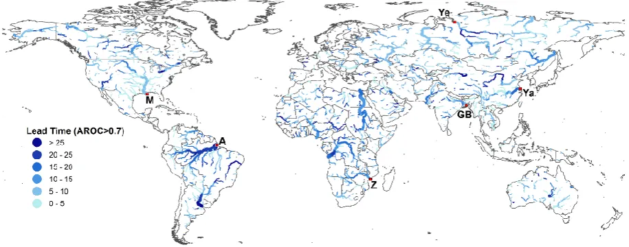
[image:9.595.309.548.296.587.2]Fig. 8. Forecast lead time, in days, for which ESPs are skillful (AROC>0.7).
Another source of error in the hydrological model is the lack of simulation of river floodplains. This is particularly visible in the largest rivers, where simulated discharge peaks occur too early and vary faster than the corresponding obser-vations (see example in Fig. 3), which follow a more gradual evolution. Recent research by Paiva et al. (2012, 2013) and Yamazaki et al. (2011) showed considerable improvement of the streamflow simulation by including backwater effects and floodplain store of water volumes interacting with the river. 4.2 Performance of the early warning system
CRPSS maps for the 2 yr of ensemble streamflow prediction (i.e., 2009–2010) were calculated for each selected forecast lead time from 1 to 45 days. CRPSS maps with lead time of 5, 15 and 25 days are shown in Fig. 7. To improve the figure readability, only river pixels with upstream area larger than 50 000 km2 are plotted. Skillful quantitative ESPs are indi-cated with blue shadings in Fig. 7 (i.e., where CRPSS>0), while in red are indicated those rivers where a reference per-sistent forecast performs quantitatively better. As expected, the CRPSS deteriorates for increasing forecast horizons, par-ticularly in smaller rivers. Poorest performance is shown in northern cold regions, mostly in Asian and North American rivers. In large river basins in inter-tropical and mid-latitude regions (e.g., Amazon, Mississippi, Congo, Nile, Paran´a), the ESPs perform better than the reference forecast, especially for longer lead times. In fact, in such rivers the runoff has very slow and delayed response. Hence for short lead times (e.g., 5 days) the difference between the ESP and a persistent forecast is not substantial. On the other hand, smaller river basins often have their highest CRPSS for shorter lead times, while it decreases fast after 15-day lead time, when no mete-orological forcing is used as input.
The threshold exceedance analysis is evaluated through the use of ROC curves and specifically the area under these
curves, which was calculated for each of the 45 daily forecast lead times. As discussed in Sect. 3.1, the threshold between events and non-events is set to the 90th percentile of the cor-rected discharge climatology. Despite being in the upper tail of the statistical distribution of annual discharge regimes, the 90th percentile is below the three flood warning thresholds of GloFAS and usually does not correspond to flooding con-ditions. However, it is important to select a discharge value that was reached at every river pixel during the 2 yr of simu-lation, so that the skill score can be calculated for the whole domain. Results of this analysis are drawn in Fig. 8, which shows the maximum lead time over which forecasts are skill-ful (i.e., AROC>0.7, as stated in Sect. 3.2). Spatial pat-tern of results in Fig. 8 is widely in agreement with those of Fig. 7. Longest lead times are found in large river basins in South America, Africa, and South Asia, with values ex-ceeding 25 days in some areas. Smaller river basins mostly achieve maximum forecast lead times around 20 days, while in some cases they are limited within 10 days. Results from the ESP as calculated by the proposed model and shown in Figs. 7 and 8 should be filtered by excluding regions where no significant river network and runoff exists. These include desert areas such as the Sahara, Arctic, Gobi, Arabian and Australian deserts, among the largest. Unexpectedly, in the lowest part of the Mississippi River, in North America, max-imum values of lead time from Fig. 8 are within 10 days, de-spite having skillful CRPSS for lead times as long as 25 days (see Fig. 7). In other words, while quantitative streamflow predictions in the Mississippi are on average rather accurate even for long lead times, high flow events above the 90th per-centiles are skillfully detected only for a shorter time horizon. The reasons for such behavior are mostly related to a delay in the discharge peak for the main event within the considered period, which occurred in autumn 2009 (see Fig. 9).
Fig. 9. ESPs (blue shades) and corrected discharge climatology (ERA-I sim) at the outlet of six major river basins (see red mark-ers in Fig. 8), for lead time of 15 (left column) and 25 days (right column).
[image:11.595.306.552.62.191.2]These are shown at the outlet of six major river basins in different climatic regions, for forecast lead times of 15 and 25 days. Outlets location and name initials of each river are shown with red markers in Fig. 8. In all cases shown, the ensemble spread is relatively narrow, as in such large river basins the runoff is mostly driven by the initial conditions and, specifically, by water already in the river network at the start of the forecast, and that is conveyed downstream by the hydrological model. At all locations the ensemble spread is larger for the longest lead time shown, reflecting the increas-ing uncertainty range as the lead time increases. However, graphs with longer forecast lead time (not shown in the arti-cle) suggest that, after reaching its maximum, the ensemble spread tends to reduce after the predicted rainfall has drained through the basin outlet. This is the consequence of using 15 days of rainfall but simulating a longer lead time, which means that the ESP spread is increasingly underestimated af-ter day 15 of simulation. In five out of six stations in Fig. 9,
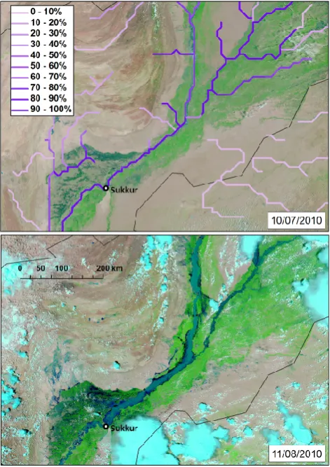
Fig. 10. 20-day ESP on 28 July 2010 for a dynamic reporting point in the Indus River near Sukkur, in Pakistan. The probability of severe threshold exceedance is shown with purple shadings. The black-contoured rectangle indicates the area shown in Fig. 12.
the runoff regime follows a clear seasonal trend, with peak flows always in the same range of months, depending on the rainfall regime and on the timing of snow and ice accumu-lation and melting. Differently, in the Mississippi River, the runoff regime is more variable and high flows occurred in different seasons. This partly explains the results shown in Fig. 7, where the ESP performs quantitatively better than a persistent forecast also for long lead times (i.e., 25 days). Graphs in Fig. 9 show that the ESP spread is higher when the hydrographs have increasing trend because of the uncer-tainty of forecast rainfall. On the other hand, as the reference simulation and the ESPs are outputs of the same hydrolog-ical model, results match very well in the recession part of the hydrographs, that is when little rainfall is forecast or dur-ing the period of snow accumulation. It is worth notdur-ing that the highest spread of the ESP occurs in the Yenisei River, where the snow and ice melting in the spring season play a prominent role in generating high flows. As a result the en-semble spread is amplified as the uncertainty of both rainfall and temperature affects the streamflow forecast.
4.3 Case study – 2010 Pakistan floods
Fig. 11. Persistence diagrams of the forecasts shown in Fig. 10, showing the probability (%) of exceeding the high and severe alert level over five consecutive forecasts issued from 24 to 28 July 2010.
River, few kilometers downstream the city of Sukkur, in the Sindh province of Pakistan. Geographic location of the area is shown by a black-contoured rectangle in Fig. 6. Forecasts show a sharp rise of discharge in the river, with expected peak of the ensemble mean on the 10 August, hence 13 days after the prediction was issued. The uncertainty range increases with the lead time, though it almost completely exceeds the severe alert level from the 8 to the 12 August. The persis-tence diagram for the same point is shown in Fig. 11, which indicates a probability larger than 50 % of exceeding the high alert level (i.e., 5 yr return period) on the 10, 11 and 12 Au-gust as early as the 24 July, thus 17 to 19 days in advance. On the other hand, the probability of exceeding the severe alert level increased considerably over five consecutive forecasts, from 16 % (24 July) to a maximum of 96 % (28 July). The following forecasts confirmed these results indicating, for the same station, a maximum probability to exceed the severe alert level of 100 % from the 7 August onwards. On 9 August, the BBC reported that the measured discharge through the Sukkur Barrage was up to 1.4 million cubic feet per second (cusecs), i.e., about 39 600 m3s−1, way higher than its de-sign capacity of 900 000 cusecs (http://www.bbc.co.uk/news/ world-south-asia-10910778). Also, Fig. 12 shows a compar-ison between satellite images taken on 10 July 2010 (top) and on 11 August 2010 (bottom) from MODIS Rapid Re-sponse (Descloitres et al., 2002) in the area delimited by the black-contoured rectangle shown in Fig. 10. In the lat-ter the extent of flooded areas (with dark shades) is clearly visible for a wide portion of the Indus River basin. In the top panel of Fig. 12, the maximum probability of exceed-ing the severe warnexceed-ing threshold over the forecast range (i.e., 20 yr return period) is indicated with purple shades (ESP of 28 July 2010).
5 Discussions and conclusions
[image:12.595.49.286.66.174.2]In this article we present a probabilistic flood early warn-ing system runnwarn-ing at global scale, aimed at forecastwarn-ing the threshold exceedance of ensemble streamflow predictions on
Fig. 12. Satellite images of the Indus River on 10 July 2010 (top) and on 11 August 2010 (bottom). Top panel also shows, with purple shadings, the maximum probability of exceeding the severe thresh-old in a 20-day forecast range (forecast on 28 July 2010).
Findings of this analysis show that current ensemble weather predictions can enable skillful detection of haz-ardous events with forecast horizon as long as 1 month in large river basins, providing that the initial conditions are es-timated correctly. This anticipation depends on the skill of input weather forecasts and on the delay between the me-teorological forcing and the hydrological response in the river basin. Interestingly, the uncertainty range of ensem-ble weather predictions has a reduced effect when propa-gated to discharge predictions in large river basins. Indeed, flood events in major rivers are mostly caused by large-scale weather systems that are skillfully predicted by state-of-the-art global forecasting models. In addition, when weather sys-tems have smaller or similar size as that of the river basin, spatial shifts of predicted rainfall fields have limited effect on the resulting streamflow at the outlet.
With regard to the system performance in quantitative forecasting and early warning, the maximum added value is shown (i) in medium-size river basins, (ii) in those with rel-atively fast response and (iii) in basins with no definite trend in the seasonal runoff. At the lower boundary of the range of basin size, forecast performance deteriorates quickly with increasing lead time and with decreasing upstream area. In-deed, in these river basins, flood events are caused by small-size weather systems that cannot be properly modeled by the current system, as the model space–time resolution is comparatively coarse for their typical hydro-meteorological dynamics. Consequently, on the basis of the analysis per-formed in this work, the authors suggest a lower boundary of 10 000 km2as the minimum upstream area to consider for streamflow predictions provided by the model.
In contrast, in the largest world river basins (i.e., basin area larger than 1 million km2)variations of river discharge occur at slow rates. Hence the 1- to 10-day streamflow prediction does not differ substantially from a persistent forecast (i.e., the last observed discharge value). On the other hand, results for these basins show skillful predictions for lead times up to one month, whereas the highest added value compared to persistent forecast is provided for lead times of 10–30 days (see Fig. 7). Besides the slow response, large river basins have long memory, so even small errors in model compo-nents such as snow accumulation and soil moisture can sum up over long time and induce a considerable bias in the water balance. An accurate estimation of the initial model state is therefore of crucial importance for the overall system perfor-mance. This can be achieved by regularly updating the water balance using the latest input data from ERA-Interim reanal-ysis, to improve the consistency between ensemble forecasts and the climatological warning thresholds. In addition, recent works in data assimilation and correction techniques demon-strated large potential for improving quantitative streamflow forecasts at those stations where discharge measurements are provided in real time (e.g., Bogner and Pappenberger, 2011). This work shows the system setup and skills in its ini-tial stage; that is, no calibration has been performed on the
hydrological model behind. This is an important step for future improvements, particularly for a global system that therefore includes the full range of climates and hydrolog-ical regimes of the earth. Results in Figs. 7–8 show the cur-rent system potential assuming that the simulated climatol-ogy corresponds to the actual river conditions, that is, for a perfect model process representation, calibration, and perfect input forcing. The presented research work shows that there is substantial room for improving the current model param-eterization, with particular focus on hydrological regimes in arid and cold regions. However, errors coming from the hy-drological modeling and from the weather predictions do not sum up linearly in the assessment of the overall system per-formance. As stated in Sect. 3.1, the main goal of an early warning system is to match the percentile rank of each sim-ulated and observed discharge, rather than optimizing quan-titative values. In addition, the model capability would also benefit from improved weather forecasts and possibly from the use of input data with longer forecast horizon. In this regard, the use of monthly ECMWF VarEPS forecasts – cur-rently issued twice per week – is envisaged for future system applications while, for the remaining five days of the week, climatological average values could represent a better alter-native to use to the current assumption of no input flow.
As a final remark, the current system is based on warning thresholds with fixed probability levels, corresponding to se-lected return periods. Actual flood risk also depends on the vulnerability of each area. For instance, in sparsely populated areas or in regions with prominent flood defense works, the 100 yr discharge may cause limited economic damage. Con-versely in densely populated areas with poor flood protection measures, peak discharges with relatively low return periods can cause severe damage. The coupling of hazard and vulner-ability maps would be extremely beneficial for this system, in order to rank warnings according to the potential economic damage that floods can cause as well as to the corresponding affected population.
Acknowledgements. We thank the Global Runoff Data Centre for providing historic discharge measurements. Also, the editor and the three reviewers are gratefully acknowledged for their valuable feedback.
Edited by: R. Woods
References
Alfieri, L., Salamon, P., Pappenberger, F., Wetterhall, F., and Thie-len, J.: Operational early warning systems for water-related haz-ards in Europe, Environ. Sci. Policy, 21, 35–49, 2012a.
Alfieri, L., Thielen, J., and Pappenberger, F.: Ensemble hydro-meteorological simulation for flash flood early detection in southern Switzerland, J. Hydrol., 424–425, 143–153, doi:10.1016/j.jhydrol.2011.12.038, 2012b.
ECMWF Model: Verification from Field Site to Terrestrial Wa-ter Storage and Impact in the Integrated Forecast System, J. Hy-drometeorol., 10, 623–643, doi:10.1175/2008JHM1068.1, 2009. Balsamo, G., Boussetta, S., Dutra, E., Beljaars, A., Viterbo, P., and Van de Hurk, B.: Evolution of land surface processes in the IFS, ECMWF Newsletter, 127, 17–22, 2011a.
Balsamo, G., Pappenberger, F., Dutra, E., Viterbo, P., and van den Hurk, B.: A revised land hydrology in the ECMWF model: a step towards daily water flux prediction in a fully-closed water cycle, Hydrol. Process., 25, 1046–1054, 2011b.
Balsamo, G., Albergel, C., Beljaars, A., Boussetta, S., Brun, E., Cloke, H., Dee, D., Dutra, E., Pappenberger, F., de Rosnay, P., Mu˜noz Sabater, J., Stockdale, T., and Vitart, F.: Interim/Land: A global land-surface reanalysis based on ERA-Interim meteorological forcing, ERA Report Series, ECMWF, Shinfield Park, Reading, 2012.
Bartholmes, J. C., Thielen, J., Ramos, M. H., and Gentilini, S.: The european flood alert system EFAS – Part 2: Statistical skill as-sessment of probabilistic and deterministic operational forecasts, Hydrol. Earth Syst. Sci., 13, 141–153, doi:10.5194/hess-13-141-2009, 2009.
Bogner, K. and Pappenberger, F.: Multiscale error analy-sis, correction, and predictive uncertainty estimation in a flood forecasting system, Water Resour. Res., 47, W07524, doi:10.1029/2010WR009137, 2011.
Buizza, R., Hollingsworth, A., Lalaurette, F., and Ghelli, A.: Probabilistic Predictions of Precipitation Using the ECMWF Ensemble Prediction System, Weather Forecast., 14, 168–189, doi:10.1175/1520-0434(1999)014<0168:PPOPUT>2.0.CO;2, 1999.
Candogan Yossef, N., van Beek, L. P. H., Kwadijk, J. C. J., and Bierkens, M. F. P.: Assessment of the potential forecasting skill of a global hydrological model in reproducing the occurrence of monthly flow extremes, Hydrol. Earth Syst. Sci., 16, 4233–4246, doi:10.5194/hess-16-4233-2012, 2012.
Carsell, K., Pingel, N., and Ford, D.: Quantifying the Benefit of a Flood Warning System, Natural Hazards Review, 5, 131–140, doi:10.1061/(ASCE)1527-6988(2004)5:3(131), 2004.
Chow, V. T., Maidment, D. R., and Mays, L. W.: Applied hydrology, McGraw-Hill Science/Engineering/Math., 1988.
Cloke, H. L. and Pappenberger, F.: Ensemble flood forecasting: A review, J. Hydrol., 375, 613–626, 2009.
CRED: EM-DAT: The OFDA/CRED International Disaster Database, available at: www.emdat.be (last access: 13 March 2013), Universit´e Catholique de Louvain, Brussels (Belgium), 2011.
de Groeve, T.: Flood monitoring and mapping using passive mi-crowave remote sensing in Namibia, Geomatics, Natural Hazards and Risk, 1, 19–35, 2010.
de Roo, A. P. J., Gouweleeuw, B., Thielen, J., Bartholmes, J., Bongioannini-Cerlini, P., Todini, E., Bates, P. D., Horritt, M., Hunter, N., Beven, K., Pappenberger, F., Heise, E., Rivin, G., Hils, M., Hollingsworth, A., Holst, B., Kwadijk, J., Reggiani, P., Van Dijk, M., Sattler, K., and Sprokkereef, E.: Development of a European flood forecasting system, International Journal of River Basin Management, 1, 49–59, 2003.
Dee, D. P., Uppala, S. M., Simmons, A. J., Berrisford, P., Poli, P., Kobayashi, S., Andrae, U., Balmaseda, M. A., Balsamo, G., Bauer, P., Bechtold, P., Beljaars, A. C. M., van de Berg, L.,
Bid-lot, J., Bormann, N., Delsol, C., Dragani, R., Fuentes, M., Geer, A. J., Haimberger, L., Healy, S. B., Hersbach, H., Holm, E. V., Isaksen, L., Kallberg, P., Kohler, M., Matricardi, M., McNally, A. P., Monge-Sanz, B. M., Morcrette, J.-J., Park, B.-K., Peubey, C., de Rosnay, P., Tavolato, C., Thepaut, J.-N., and Vitart, F.: The ERA-Interim reanalysis: configuration and performance of the data assimilation system, Q. J. Roy. Meteorol. Soc., 137, 553– 597, doi:10.1002/qj.828, 2011.
Descloitres, J., Sohlberg, R., Owens, J., Giglio, L., Justice, C., Car-roll, M., Seaton, J., Crisologo, M., Finco, M., and Lannom, K.: The MODIS rapid response project, in: Geoscience and Remote Sensing Symposium, IGARSS’02: IEEE International, Vol. 2, 1191–1192, available at: http://ieeexplore.ieee.org/xpls/abs all. jsp?arnumber=1025879 (last access: 10 January 2013), 2002. Dutra, E., Balsamo, G., Viterbo, P., Miranda, P. M. A., Beljaars,
A., Schar, C., and Elder, K.: An improved snow scheme for the ECMWF land surface model: Description and offline validation, J. Hydrometeorol., 11, 899–916, 2010.
European Commission: Council Regulation (EC) No 2012/2002 of 11 November 2002 establishing the European Union Solidarity Fund, 2002.
Fekete, B. M., V¨or¨osmarty, C. J., and Lammers, R. B.: Scaling gridded river networks for macroscale hydrology: Development, analysis, and control of error, Water Resour. Res., 37, 1955– 1967, doi:10.1029/2001WR900024, 2001.
Feyen, L., Vrugt, J. A., Nuall´ain, B. ˜A., van der Knijff, J., and De Roo, A.: Parameter optimisation and uncertainty assessment for large-scale streamflow simulation with the LISFLOOD model, J. Hydrol., 332, 276–289, doi:10.1016/j.jhydrol.2006.07.004, 2007.
Fundel, F. and Zappa, M.: Hydrological ensemble forecast-ing in mesoscale catchments: Sensitivity to initial conditions and value of reforecasts, Water Resour. Res., 47, W09520, doi:10.1029/2010WR009996, 2011.
Guha-Sapir, D., Vos, F., Below, R., and Ponserre, S.: Annual Dis-aster Statistical Review 2011: The Numbers and Trends, CRED, Brussels, 2012.
Hagen, E. and Lu, X.: Let us create flood hazard maps for develop-ing countries, Nat. Hazards, 58, 841–843, doi:10.1007/s11069-011-9750-7, 2011.
Hanssen, A. W. and Kuipers, W. J. A.: On the Relationship Be-tween the Frequency of Rain and Various Meteorological Param-eters: (with Reference to the Problem of Objective Forecasting), Staatsdrukkerij-en Uitgeverijbedrijf, available at: http://library. wur.nl/WebQuery/clc/470648 (last access: 10 January 2013), 1965.
He, Y., Wetterhall, F., Bao, H., Cloke, H., Li, Z., Pappenberger, F., Hu, Y., Manful, D., and Huang, Y.: Ensemble forecasting us-ing TIGGE for the July–September 2008 floods in the Upper Huai catchment: a case study, Atmos. Sci. Lett., 11, 132–138, doi:10.1002/asl.270, 2010.
Hersbach, H.: Decomposition of the continuous ranked probabil-ity score for ensemble prediction systems, Weather Forecast., 15, 559–570, 2000.
Huffman, G. J., Adler, R. F., Bolvin, D. T., and Gu, G.: Improving the global precipitation record: GPCP version 2.1, Geophys. Res. Lett., 36, L17808, 2009.
IFRC: The Red Cross Red Crescent approach to disaster and crisis management, Position paper, Geneva, 2011.
Lehner, B., Verdin, K., and Jarvis, A.: New Global Hydrography Derived From Spaceborne Elevation Data, Eos T. Am. Geophys. Un., 89, 93–94, doi:200810.1029/2008EO100001, 2008. Loveland, T. R., Reed, B. C., Brown, J. F., Ohlen, D. O., Zhu, Z.,
Yang, L., and Merchant, J. W.: Development of a global land cover characteristics database and IGBP DISCover from 1 km AVHRR data, Int. J. Remote Sens., 21, 1303–1330, 2000. Marzban, C.: The ROC curve and the area under it as performance
measures, Weather Forecast., 19, 1106–1114, 2004.
Miller, M., Buizza, R., Haseler, J., Hortal, M., Janssen, P., and Untch, A.: Increased resolution in the ECMWF deterministic and ensemble prediction systems, ECMWF Newsletter, 124, 10–16, 2010.
Nester, T., Komma, J., Viglione, A., and Bl¨oschl, G.: Flood forecast errors and ensemble spread – A case study, Water Resour. Res., 48, W10502, doi:10.1029/2011WR011649, 2012.
Paiva, R. C. D., Collischonn, W., Bonnet, M. P., and de Gonc¸alves, L. G. G.: On the sources of hydrological prediction uncer-tainty in the Amazon, Hydrol. Earth Syst. Sci., 16, 3127–3137, doi:10.5194/hess-16-3127-2012, 2012.
Paiva, R. C. D., Buarque, D. C., Collischonn, W., Bonnet, M.-P., Frappart, F., Calmant, S., and Mendes, C. A. B.: Large-scale hydrologic and hydrodynamic modelling of the Amazon River basin, Water Resour. Res., online first, doi:10.1002/wrcr.20067, 2013.
Pappenberger, F., Cloke, H. L., Balsamo, G., Ngo-Duc, T., and Oki, T.: Global runoff routing with the hydrological component of the ECMWF NWP system, Int. J. Climatol., 30, 2155–2174, 2010a. Pappenberger, F., Thielen, J., and Del Medico, M.: The impact of weather forecast improvements on large scale hydrology: analysing a decade of forecasts of the European Flood Alert Sys-tem, Hydrol. Process., 25, 1091–1113, doi:10.1002/hyp.7772, 2010b.
Pappenberger, F., Dutra, E., Wetterhall, F., and Cloke, H. L.: Deriv-ing global flood hazard maps of fluvial floods through a phys-ical model cascade, Hydrol. Earth Syst. Sci., 16, 4143–4156, doi:10.5194/hess-16-4143-2012, 2012.
Prinos, P., Kortenhaus, A., Swerpel, B., and Jim´enez, J. A.: Review of Flood Hazard Mapping, available at: http://www.floodsite.net/html/partner area/project docs/ T03 07 01 Review Hazard Mapping V4 3 P01.pdf (last access: 28 September 2012), 2008.
Proud, S. R., Fensholt, R., Rasmussen, L. V., and Sandholt, I.: Rapid response flood detection using the MSG geostationary satellite, Int. J. Appl. Earth Obs., 13, 536–544, 2011.
Rao, C. X. and Maurer, E. P.: A simplified model for predicting daily transmission losses in a stream channel, J. Am. Water Re-sour. As., 32, 1139–1145, 1996.
Sperna Weiland, F. C., van Beek, L. P. H., Kwadijk, J. C. J., and Bierkens, M. F. P.: The ability of a GCM-forced hydro-logical model to reproduce global discharge variability, Hy-drol. Earth Syst. Sci., 14, 1595–1621, doi:10.5194/hess-14-1595-2010, 2010.
Thielen, J., Bartholmes, J., Ramos, M.-H., and de Roo, A.: The Eu-ropean Flood Alert System – Part 1: Concept and development, Hydrol. Earth Syst. Sci., 13, 125–140, doi:10.5194/hess-13-125-2009, 2009a.
Thielen, J., Bogner, K., Pappenberger, F., Kalas, M., del Medico, M., and de Roo, A.: Monthly-, medium-, and short-range flood warning: Testing the limits of predictability, Meteorol. Appl., 16, 77–90, 2009b.
Thiemig, V., Pappenberger, F., Thielen, J., Gadain, H., de Roo, A., Bodis, K., Del Medico, M., and Muthusi, F.: Ensemble flood forecasting in Africa: A feasibility study in the Juba-Shabelle river basin, Atmos. Sci. Lett., 11, 123–131, 2010.
Trenberth, K. E., Dai, A., Rasmussen, R. M., and Parsons, D. B.: The changing character of precipitation, B. Am. Meteorol. Soc., 84, 1205–1217, 2003.
UN/ISDR: Living with risk: A global review of disaster reduction initiatives, ISDR Secretariat, Geneva, Switzerland., 2002. van der Knijff, J. M., Younis, J., and de Roo, A. P. J.: LISFLOOD: A
GIS-based distributed model for river basin scale water balance and flood simulation, Int. J. Geogr. Inf. Sci., 24, 189–212, 2010. Voisin, N., Schaake, J. C., and Lettenmaier, D. P.: Calibra-tion and Downscaling Methods for Quantitative Ensemble Precipitation Forecasts, Weather Forecast., 25, 1603–1627, doi:10.1175/2010WAF2222367.1, 2010.
Voisin, N., Pappenberger, F., Lettenmaier, D. P., Buizza, R., and Schaake, J. C.: Application of a Medium-Range Global Hydrologic Probabilistic Forecast Scheme to the Ohio River Basin, Weather Forecast., 26, 425–446, doi:10.1175/WAF-D-10-05032.1, 2011.
Wang, J., Hong, Y., Li, L., Gourley, J. J., Khan, S. I., Yilmaz, K. K., Adler, R. F., Policelli, F. S., Habib, S., Irwn, D., Limaye, A. S., Korme, T., and Okello, L.: The coupled routing and excess storage (CREST) distributed hydrological model, Hydrolog. Sci. J., 56, 84–98, doi:10.1080/02626667.2010.543087, 2011. Westerhoff, R. S., Kleuskens, M. P. H., Winsemius, H. C., Huizinga,
H. J., Brakenridge, G. R., and Bishop, C.: Automated global water mapping based on wide-swath orbital synthetic-aperture radar, Hydrol. Earth Syst. Sci., 17, 651–663, doi:10.5194/hess-17-651-2013, 2013.
Wilks, D. S.: Statistical Methods in the Atmospheric Sciences: An Introduction, electronic version., Elsevier, San Diego, CA, avail-able at: http://cdsweb.cern.ch/record/992087 (last access: 7 Oc-tober 2010), 2006.
Winsemius, H. C., Van Beek, L. P. H., Jongman, B., Ward, P. J., and Bouwman, A.: A framework for global river flood risk assessments, Hydrol. Earth Syst. Sci. Discuss., 9, 9611–9659, doi:10.5194/hessd-9-9611-2012, 2012.
Wu, H., Adler, R. F., Hong, Y., Tian, Y., and Policelli, F.: Eval-uation of Global Flood Detection Using Satellite-Based Rain-fall and a Hydrologic Model, J. Hydrometeorol., 13, 1268–1284, doi:10.1175/JHM-D-11-087.1, 2012a.
Wu, H., Kimball, J. S., Li, H., Huang, M., Leung, L. R., and Adler, R. F.: A new global river network database for macroscale hydrologic modeling, Water Resour. Res., 48, W09701, doi:10.1029/2012WR012313, 2012b.