Are we using the right fuel to drive hydrological models? A climate impact study in the Upper Blue Nile

(1)

Are we using the right fuel to drive hydrological models?

A climate impact study in the Upper Blue Nile

Stefan Liersch1_{, Julia Tecklenburg}1_{, Henning Rust}2_{, Andreas Dobler}2_{, Madlen Fischer}2_{, Tim Kruschke}3_,

Hagen Koch1_{, and Fred Fokko Hattermann}1

1_{Potsdam Institute for Climate Impact Research (PIK), Telegraphenberg A31, 14473 Potsdam, Germany}

2_{Free University of Berlin (FUB), Institute of Meteorology, Carl-Heinrich-Becker-Weg 6–10, 12165 Berlin, Germany} 3_{GEOMAR Helmholtz Centre for Ocean Research Kiel, Wischhofstr. 1–3, 24148 Kiel, Germany}

Correspondence:Stefan Liersch ([email protected]) Received: 18 August 2016 – Discussion started: 26 September 2016

Revised: 23 October 2017 – Accepted: 11 December 2017 – Published: 9 April 2018

Abstract. Climate simulations are the fuel to drive hydro-logical models that are used to assess the impacts of climate change and variability on hydrological parameters, such as river discharges, soil moisture, and evapotranspiration. Un-like with cars, where we know which fuel the engine re-quires, we never know in advance what unexpected side ef-fects might be caused by the fuel we feed our models with. Sometimes we increase the fuel’s octane number (bias cor-rection) to achieve better performance and find out that the model behaves differently but not always as was expected or desired. This study investigates the impacts of projected cli-mate change on the hydrology of the Upper Blue Nile catch-ment using two model ensembles consisting of five global CMIP5 Earth system models and 10 regional climate mod-els (CORDEX Africa). WATCH forcing data were used to calibrate an eco-hydrological model and to bias-correct both model ensembles using slightly differing approaches. On the one hand it was found that the bias correction methods con-siderably improved the performance of average rainfall char-acteristics in the reference period (1970–1999) in most of the cases. This also holds true for non-extreme discharge conditions between Q₂₀ andQ₈₀. On the other hand,

bias-corrected simulations tend to overemphasize magnitudes of projected change signals and extremes. A general weakness of both uncorrected and bias-corrected simulations is the rather poor representation of high and low flows and their extremes, which were often deteriorated by bias correction. This inaccuracy is a crucial deficiency for regional impact studies dealing with water management issues and it is there-fore important to analyse model performance and

character-istics and the effect of bias correction, and eventually to ex-clude some climate models from the ensemble. However, the multi-model means of all ensembles project increasing av-erage annual discharges in the Upper Blue Nile catchment and a shift in seasonal patterns, with decreasing discharges in June and July and increasing discharges from August to November.

1 Introduction

Ethiopia is a country where about 80 % of the population is engaged in the agricultural sector (Dile et al., 2013; Deressa et al., 2011), the main source of income for rural communi-ties (Bryan et al., 2009). Around 90 % of the country’s grain is produced by smallholder farms. Subsistence and rain-fed farming systems dominate and, with few exceptions, irriga-tion is not practised1_{. Consequently, agricultural and}

live-stock production, people’s livelihoods, and food security de-pend strongly on weather conditions, mainly on rainfall pat-terns such as amounts and timing. Hence, a large share of Ethiopia’s population is very vulnerable to weather condi-tions and in particular to its inter-annual variability (Busby et al., 2014; Megersa et al., 2014; Headey et al., 2014; Za-itchik et al., 2012; Simane et al., 2012).

The Ethiopian highlands, where the Blue Nile rises, are considered to be the “water tower” of East Africa. The Blue Nile, for instance, contributes about 55–65 % of the flow of the Nile at the confluence with the White Nile (King, 2013;

(2)

Sutcliffe and Parks, 1999). The river is therefore the most important water resource, not only for Ethiopia but also for the downstream riparian countries of Sudan and Egypt. Wa-ter politics in the Nile basin have a long history and are a central geopolitical feature in this region (Gebreluel, 2014; Ibrahim, 2012). With growing populations, industrialization, and climate change and its variability, the situation is be-coming more and more tense (Gebreluel, 2014). Knowledge about availability of future water resources in this region and therefore studies providing insights into climate change and variability, and their impacts on hydrology, are of utmost im-portance.

A review of future hydrological and climate studies in the River Nile basin is provided by Di Baldassarre et al. (2011) and a review on hydrological extremes in the Upper Blue Nile catchment (UBN) by Taye et al. (2015). Recent stud-ies on climate change and variability in the UBN or its trib-utaries served different purposes. The studies by Mengistu et al. (2014), Taye and Willems (2012), Conway and Schip-per (2011), and Conway and Hulme (1993) investigated for instance trends of past climate change using observed and/or generated climate data. Diro et al. (2009) analysed the qual-ity of rainfall data using two numerical weather prediction models. Another category of studies investigates the perfor-mance and projected trends of climate models (e.g. Conway and Schipper, 2011; Diro et al., 2011).

Studies performed to assess impacts of climate change in the UBN can be categorized into (i) studies applying simple approaches, assuming for instance a fixed percentage of de-crease or inde-crease of a climatic variable or discharge (Jeuland and Whittington, 2014); (ii) studies using a single climate model (e.g. McCartney and Menker Girma, 2012; Soliman et al., 2009; Abdo et al., 2009); and (iii) studies analysing complex climate model ensembles (e.g. Teklesadik et al., 2017; Liersch et al., 2017; Aich et al., 2014; Mengistu and Sorteberg, 2012; Setegn et al., 2011; Beyene et al., 2010; Elshamy et al., 2009; Kim et al., 2008).

As a matter of fact, climatic variables such as air temper-ature, precipitation, and radiation simulated by global and regional climate models usually have a bias in the historical (reference) period (e.g. Addor and Seibert, 2014; Berg et al., 2012; Gudmundsson et al., 2012; Hagemann et al., 2011). Moreover, they often fail to adequately represent spatio-temporal dynamics at the regional scale. In climate studies, the absolute or relative changes between historical and pro-jection periods are analysed and reported in the following manner: model X projects a temperature increase of 2.5 K in 2021–2050 and an increase of 8 % of rainfall relative to its reference period. Here, it does not matter whether model X was too cold/warm or too dry/wet during the reference pe-riod. Only the rate of change matters, which might be rea-sonable in this context. Moreover, in climate change studies it is common practice nowadays to analyse the entire avail-able model ensemble and to calculate the multi-model mean, which is superior to any one individual climate model (Pierce

et al., 2009). Unfortunately, a daily multi-model mean cli-mate time series does not serve as reasonable input for impact models operating at the daily time step. Therefore, the appli-cation of climate model ensembles is always recommended for hydrological studies (Teutschbein and Seibert, 2010) and is considered nowadays as state of the art.

Quantitative and application-oriented impact studies re-quire a certain accuracy of input data as well as adequate representation of the relevant processes by the models used. Small biases already present in temperature or precipitation may lead to considerable biases in impact models (Maraun et al., 2010). Therefore, various bias correction approaches were developed, particularly for hydrological applications (Piani et al., 2010; Dosio and Paruolo, 2011). The expecta-tion of using bias-corrected input data is that they are quan-titatively more precise than their uncorrected counterparts.

The authors of studies using complex model ensembles in the UBN, cited above, applied different approaches to gen-erate climate input time series for hydrological modelling. Elshamy et al. (2009) used a distribution mapping approach to simultaneously downscale and bias-correct 17 CMIP32 GCMs (SRES A1B) and applied the corrected climate data to run the Nile Forecasting System in the UBN. The delta-change method was used by Mengistu and Sorteberg (2012) and Kim et al. (2008) to generate time series of tempera-ture and precipitation used as input for hydrological mod-elling. Mengistu and Sorteberg (2012) used 19 GCMs of the CMIP3 model ensemble (SRES scenarios A2, A1B, and B1) to generate climate inputs for the SWAT model and Kim et al. (2008) used six GCMs (SRES A2) to run a monthly water balance model. Setegn et al. (2011) applied a downscaling approach for daily temperature and precipitation data to 15 CMIP3 GCMs (SRES scenarios A2, A1B, and B1) using a cumulative frequency distribution approach. They used the climate data to run the SWAT model in the Lake Tana basin. Beyene et al. (2010) performed a quantile mapping approach to bias-correct 11 CMIP3 GCMs (SRES A2 and B1) to run the VIC hydrological model for the entire Nile basin. Re-cently, Teklesadik et al. (2017) published a study comparing climate change impacts, particularly on actual evapotranspi-ration, using six hydrological models driven by the same four CMIP5 GCMs used in the study at hand. Liersch et al. (2017) used a climate model ensemble to analyse the impacts of the Grand Ethiopian Renaissance Dam on downstream dis-charges under current and future climate conditions based on the 10 “best” global and regional climate models identified in this study.

The study at hand falls into the same category using the most recent global and regional climate projections released for the IPCC 5th Assessment Report (IPCC, 2013). Uncor-rected and bias-corUncor-rected climate simulations of five CMIP53

2_{http://cmip-pcmdi.llnl.gov/cmip3_overview.html?} submenuheader=1

(3)

Earth system models (ESMs) and 10 uncorrected and bias-corrected regional climate models (RCMs) from CORDEX Africa4_{were used to run the Soil and Water Integrated Model}

(SWIM). The climate scenarios used by both model ensem-bles are the Representative Concentration Pathways (RCPs) RCP 4.5 and RCP 8.5 (van Vuuren et al., 2011; Meinshausen et al., 2011). Hence, we analyse 60 discharge simulations (two RCPs and 15 uncorrected and 15 bias-corrected climate model runs) for the reference period 1970–1999 and two fu-ture periods 2030–2059 and 2070–2099.

The first objective of this study is to assess climate change and its impacts on the availability of future water resources in the UBN defined at gauge El Diem (Sudan border). The second objective is to discuss the implications of using dif-ferent model ensembles to project future discharges by com-paring the results of the whole range of uncorrected and bias-corrected ESMs and RCM ensembles. Eventually an ensem-ble is assemensem-bled including only those members fulfilling cer-tain performance criteria. These criteria are used to character-ize the suitability of simulations for different purposes, such as for qualitative or quantitative studies. A qualitative impact study may have lower demands on the quality of climate sim-ulations than a study investigating hydrological extremes or water management strategies. In the latter case, the require-ments in terms of quantitative accuracy are much higher. The following questions were central to our investigations.

a. What are the likely impacts of climate change on future discharges in the UBN?

b. Is there an agreement on the signal of climate change impacts in the 21st century using different climate model ensembles?

c. To what extent can bias correction alter the magnitudes of change signals in hydrological simulations in the study area?

d. In how far can we trust simulations that require a strong correction?

2 Study area

The entire Blue Nile River basin covers an area of about 296 000 km2_{. The study area considered here is the Upper}

Blue Nile catchment (UBN) defined at gauge El Diem at the border between Ethiopia and Sudan that covers an area of 172 000 km2_{. Elshamy et al. (2009) estimates a catchment}

area of 185 000 km2_{and Mengistu and Sorteberg (2012) an}

area of 174 000 km2_{for the UBN. These discrepancies are}

certainly based on different digital elevation models and GIS algorithms used to delineate the catchment area and thus may add to the uncertainties of such studies, which are not easily

4_{http://start.org/cordex-africa/about/}

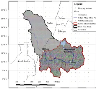
quantifiable. In Fig. 1, the UBN is encircled by a red line. In addition, it shows the 576 subbasins that were delineated for the hydrological modelling exercise, the three gauging stations used to calibrate the hydrological model, and the co-ordinates of the climate data grid. The source of the Blue Nile River is Lake Tana in the Ethiopian highlands and the catchment is located in the north-western part of Ethiopia (Taye and Willems, 2012). It drains a major part of the west-ern highlands (Sutcliffe and Parks, 1999) that is predomi-nantly governed by a unimodal rainfall regime depending on the movement of the intertropical convergence zone (ITCZ). The inter-annual variability of annual rainfall amounts in the Ethiopian highlands is high (Zaitchik et al., 2012) and ranges between 800 and 2200 mm, and the elevation of the UBN varies from 4000 to 500 m.a.s.l. (Taye and Willems, 2012). The river has a length of almost 1000 km from the Lake Tana outlet to the Sudan border.

3 Methods 3.1 Data

Freely available WATCH Forcing Data (WFD) (Weedon et al., 2011) based on ERA-40 (Uppala et al., 2005) reanal-ysis and climate observations were used to bias-correct five ESMs and 10 RCM runs and to calibrate and validate the hy-drological model SWIM (Soil and Water Integrated Model), developed by Krysanova et al. (2005). Although the qual-ity of WFD varies in space (Rust et al., 2015), this grid-ded product with a spatial resolution of 0.5◦ _{was used as}

input because observed climate data were not available for this study. The SRTM digital elevation model (Jarvis et al., 2008) was used to delineate the 576 subbasins and to derive some terrain-specific parameters. Required soil parameters were derived from the Digital Soil Map of the World (FAO et al., 2009) and land use cover data were reclassified from Global Land Cover (GLC2000) (Bartholomé and Belward, 2005). Observed monthly discharge data for model calibra-tion and validacalibra-tion were provided by the Global Runoff Data Centre (GRDC5).

3.2 Hydrological model

The Soil and Water Integrated Model (SWIM), developed by Krysanova et al. (2005), is a semi-distributed, process-based eco-hydrological model that operates at the daily time step. It was developed on the basis of the MATSALU (Krysanova et al., 1989) and SWAT (Arnold et al., 1993) models and is continuously being further developed and adapted to new or specific requirements (Krysanova et al., 2015). Hydrologi-cal response units (HRUs), considered as areas with simi-lar hydrological characteristics, are the smallest model units where all hydrological, nutrient, and vegetation processes

(4)

[image:4.612.135.461.66.366.2]

Figure 1.Map of the Blue Nile River basin. The Upper Blue Nile (UBN) catchment (172 000 km2) is enclosed by the red line. The three gauges used for model calibration and validation are represented by white circles.

are calculated. There is no lateral interaction between HRUs but area-weighted daily fluxes are calculated and aggregated at the subbasin scale and routed through the river network. SWIM distinguishes three flow components: surface runoff, subsurface runoff, and contributions of the shallow ground-water aquifer. Actual evapotranspiration is determined by simulated soil evaporation and transpiration from the vege-tation cover. Water percolating from the shallow groundwa-ter aquifer into the deep groundwagroundwa-ter aquifer is lost from the system but is considered in the water balance.

A reservoir module, developed by Koch et al. (2013), was incorporated in SWIM and parameterized to better account for Lake Tana’s storage effects and to consider the impact of the weir at the lake’s outlet in future simulations that was constructed in the year 1996.

Radiation data required by SWIM as essential climate in-put were not available in all RCM runs. To maintain consis-tency and comparability in hydrological simulations, daily radiation data were computed after Hargreaves and Samani (1985) from daily minimum and maximum air temperature and the latitude of the respective subbasin. The simulated ra-diation data were calibrated to fit average annual observed radiation data of about 1800 kWh m−₂_.

3.3 Climate models

The ESM ensemble used in this study consists of the fol-lowing five CMIP5 models: GFDL-ESM2M, HadGEM2-ES, IPSL-CM5A-LR, MIROC-ESM-CHEM, and NorESM1-M. Projections of these five ESMs were linearly downscaled and bias-corrected by Hempel et al. (2013) in the frame of the Inter-Sectoral Impact Model Intercomparison Project (ISIMIP)6_{(Warszawski et al., 2014). The uncorrected ESM}

simulations were interpolated to the WFD 0.5◦_grid.

Table S1 in the Supplement provides an overview of the RCM runs organized by the CORDEX Africa initiative7_{. The}

ensemble consists of four RCMs driven by different ESMs. The RCM SMHI-RCA4 was driven by seven ESMs, Can-RCM4 by CanESM2, and the RCMs KNMI-RACMO22T and DMI-HIRHAM4 by EC-EARTH. The 10 RCM runs were bias-corrected by the authors of this paper. Table S2 shows the model IDs of all 15 climate models used in some figures and tables.

6_{https://www.pik-potsdam.de/research/} climate-impacts-and-vulnerabilities/research/ rd2-cross-cutting-activities/isi-mip

(5)

3.4 Climate scenarios

For both the global and regional climate model ensembles, the two scenarios RCP 4.5 and RCP 8.5 were used because they represent a broad range of uncertainties with regard to possible future pathways and related climate projections. According to van Vuuren et al. (2011) and Meinshausen et al. (2011), RCP 4.5 represents the medium stabilization scenario (stabilization without overshoot pathway leading to

+4.5 W m−2radiative forcing (relative to pre-industrial

forc-ing) and ∼650 ppm CO₂equiv. by 2100) and RCP 8.5 the

highest emission scenario (rising radiative forcing pathway leading to +8.5 W m−2 and∼1370 ppm CO₂eq. by 2100),

assuming no stabilization in global greenhouse gas emis-sions.

3.5 Bias correction

Despite regional downscaling to finer resolution, RCM sim-ulations often show considerable biases when compared to observed data (Addor and Seibert, 2014; Christensen et al., 2008). A review of bias correction methods (linear scaling, local intensity scaling, power transformation, and distribu-tion or quantile mapping) is provided by Teutschbein and Seibert (2012). The authors conclude that the distribution or quantile mapping method achieves the best performance for most of the selected criteria. Although quantile mapping is a successful method to improve the representation of daily rainfall characteristics, it fails to correct multi-day and inter-annual variables, such as mean maximum 4-day precipita-tion, mean minimum 14-day precipitaprecipita-tion, and inter-annual variability (Addor and Seibert, 2014). The drawback that all approaches have in common is that they are based on the stationarity assumption, which presumes that future physi-cal processes in the atmosphere are comparable to the period used to correct the simulations. Bias correction of climate simulation data is nowadays a widely used practice in hydro-logical impact modelling, but it should be treated with cau-tion. As Maraun et al. (2010) point out, the origins of the bias in climate simulations (mathematical formulations in climate models) are not solved by the post-processing and may dis-rupt internal physical coherence between weather variables. Hence, the correction is usually based on wrong reasons (Ad-dor and Seibert, 2014). Alternatives to bias correction are so-called delta-change methods. Sophisticated approaches of this method are described by Anandhi et al. (2011), Bosshard et al. (2011), and Chiew et al. (2009).

3.5.1 Bias correction of ESMs

Bias-corrected data of five CMIP5 ESMs were available and provided by ISIMIP. In a first step ESM data were linearly in-terpolated to the WFD 0.5◦_{grid, implementing the standard}

Gregorian calendar. Temperature data were corrected using a trend-preserving additive approach where monthly mean

values were adjusted for a systematic bias by adding a grid-point-specific and month-specific constant offset. Therefore, the absolute projected temperature changes of the ESMs are not changed. The daily variability of ESM temperatures was adjusted to reproduce WFD variability by adding a monthly correction factor on temperature anomalies.

Precipitation data were corrected using a multiplicative ap-proach where monthly mean precipitation was multiplied by a grid-point-specific and month-specific constant correction factor. Relative changes projected by the ESMs are thereby preserved. A known problem of this method is that extraordi-narily high values of daily precipitation can occur in the bias-corrected simulation if very high simulated daily precipita-tion data are multiplied by high correcprecipita-tion factors. Therefore, the correction factor was limited to a value of 10. Remaining extremely high daily precipitation values were truncated to 400 mm. After the method introduced by Piani et al. (2010), daily precipitation variability and the frequency of dry days were corrected by applying a transfer function to fit the nor-malized simulated time series of wet months to the normal-ized WFD time series. A more detailed description of the bias correction procedure applied to the five CMIP5 ESMs used in this study is provided by Hempel et al. (2013).

3.5.2 Bias correction of RCMs

Precipitation biases in most CORDEX RCMs show a high seasonality for grid boxes within the evaluation domain of the UBN. This limits a bias correction based on seasonal or annual means. However, as some of these grid boxes do show almost no precipitation events for single months, a harmonic-based bias correction method analogous to the one applied to temperature is not feasible for precipitation. Furthermore, this results in a large uncertainty in the estimation of the cor-responding monthly biases. Thus, based on the recommen-dation from Dobler and Ahrens (2008), a bias correction is only applied on months and grid boxes with more than 100 rainy days (rainfall above 1 mm day−1_{) within the calibration}

period (1951–2001).

The method applied is based on a local rainy day inten-sity scaling, correcting the frequency of rainy days and the mean precipitation on rainy days to fit the observed values in a specific calibration period (Schmidli et al., 2006). Details on the implementation and an evaluation are given in Dobler and Ahrens (2008). The method has been successfully ap-plied before as a downscaling and bias-correcting method for precipitation in alpine regions (Dobler and Ahrens, 2008; Dobler et al., 2011).

(6)

The seasonality in the location parameter of a quantity (i.e. the expectation value in the case of a Gaussian distribution) can be modelled as

µ(t )=µ0+

K

X

k=1

µksin(k ω t )+ L

X

l=1

µlcos(l ω t ), (1)

withω=₃₆₅2π

.25,t=1, . . .,366 being the time variable

run-ning over all possible days of the year;KandLare the orders

of the harmonic function expansion forµ. A scale parameter σ can be modelled analogously in this framework. The

re-sult is a climatological distribution, i.e. a description of the probability distribution throughout the year.

Selection of ordersK andLis based on a 10-fold cross

validation using the Continuous Rank Probability Score (CRPS, Wilks, 2011) as the cost function. The difference in parameters between the RCM reference and the observa-tional product (WFD) is subtracted from the parameters of the RCM projections for bias correction. Quantile mapping (e.g. Vrac and Friederichs, 2015) now maps the values from the uncorrected to the corrected climatological distribution.

Particular care needs to be taken when correcting min-imum and maxmin-imum temperature to avoid inconsistencies such asT_max< T_min. Here, a variable transformation ensures

physical consistency:

T₁=log(T_max−T ) (2)

T₂=log(T−T_min). (3)

After bias-correcting T₁ andT₂, corrected values for T_max

andT_mincan be obtained by back-transforming the variables.

3.6 Evaluating the suitability of climate simulations Evaluating the suitability of climate simulations for regional impact studies is a process that includes seemingly objective components (e.g. analysing performance criteria) and subjec-tive components (choosing criteria and setting their thresh-olds). Data visualization and interpretation by the user might be considered as a mixture of both objectivity and subjectiv-ity. The choice of periods used as reference and future projec-tion does also influence the results. The former is often pre-determined by data availability or conventions and the latter usually by the client. Moreover, there are uncertainties with regard to the quality of the dataset used as the comparison baseline, mostly observed and/or generated climate data.

Evaluation of climate model performance is complicated by the fact that climate simulations cannot be compared to the reference dataset on a real-time daily, monthly, or an-nual basis, as is common practice with discharge simulations in hydrological modelling. Climate simulations are not sup-posed to reproduce or predict the weather for a certain day, month, or year. Hence, only statistical parameters, summa-rized over a period of usually 30 years (e.g. the annual cycle represented by average daily or monthly time series), or the

mean, quantile values, and standard deviation of the entire daily time series can be used as a basis for comparison.

In the first step of climate model evaluation, daily and monthly precipitation characteristics of uncorrected (UC) and bias-corrected (BC) climate simulations were compared to WFD characteristics (reference climate). In a second step, SWIM was employed to simulate daily discharge using all climate simulations for reference and future periods. Since the main purpose of this study is to assess climate change impacts on hydrology, using hydrological performance indi-cators to evaluate climate simulations is a straightforward method. A similar approach was used by Elshamy et al. (2013) who used a GLUE-like methodology to exclude and weigh climate model performance. Another benefit of this approach is that a spatially semi-distributed hydrological model does not only account for temporal but also for spa-tial patterns of climate inputs. Therefore, the annual cycle represented by daily (n=365) discharge simulations (sim),

averaged over the 30-year reference period, was compared against the baseline simulation using WFD (ref). The perfor-mance criteria applied to these time series are the coefficient of determination (R2), PBIAS, standard deviation (SD), and

the normalized SD of discrepancies (SDD) or the centred root

mean square errors.

The characteristics of daily discharges were analysed us-ing flow duration curves (FDCs), where every sus-ingle dis-charge value is related to the percentage of time it is equalled or exceeded (Smakhtin, 2000). FDCs summarize discharge variability of a time series and display the complete range from low flows to flood events. In order to analyse and visual-ize average, low, and high flow characteristics, 17 percentile values (Q0.01–Q99.99) were used to compute FDCs based on

the entire daily discharge time series of the 30-year reference period. This method was applied to assess whether model performance is suitable to study non-extreme discharge con-ditions (NED) and/or high and low flow situations as well as their extremes.

PBIAS=

n

P

i=1

(simi−refi)·100 n

P

i=1 (refi)

(4)

SDD=SD(simi−refi)

SDref (5)

(7)

def-inition of threshold values is somewhat subjective and was influenced by the simulation results of the model ensemble. However, if the thresholds had been set more critically, al-most no climate model would have passed the evaluation pro-cess sucpro-cessfully. The model selection propro-cess and the def-inition of criteria thresholds are described in the following section.

3.7 Model selection

Beside analysing the impact of climate projections on future discharges using the whole UC and BC ESM and RCM en-sembles, a climate model ensemble was assembled contain-ing only those models that fulfil the criteria and their thresh-olds defined below. In order to become a member of the se-lected ensemble, a model must basically achieve all the fol-lowing three criteria.

– Seasonality. The annual cycle based on average daily

discharge simulations must achieveR2≥0.85. Models

withR2<0.85 are assumed to represent discharge

sea-sonality only poorly.

– Volumetric deviation. Average daily discharge

simula-tions must achieve a PBIAS≤ ±30 %.

– Non-extreme discharges (NED). NED represent

dis-charge conditions between FDC percentile values be-tween > Q₁₀ and < Q₉₀ (Q₂₀, Q₃₀, . . ., Q₈₀).

Per-centiles in this range should not deviate more than

±30 % from WFD discharge simulation.

Models meeting these three criteria are assumed to be suitable for a qualitative impact assessment and are indi-cated in the column ”pre” (preselection) in Table 1. In addi-tion, the columns HF (high flows, FDC percentilesQ₁₀,Q₅, Q₁,Q₀.1,Q0.01) and LF (low flows, FDC percentilesQ90,

Q₉₅,Q₉₉,Q₉₉.9,Q99.99) indicate further whether a

partic-ular model adequately represents extreme discharge condi-tions and might be used for specific investigacondi-tions. Again, the FDC values in the respective range should not exceed the threshold of±30 %.

After simulating discharges using all climate scenarios it was found that several simulations project enormous increase in annual river discharge already in the period 2030–2059. This was particularly the case in simulations where bias cor-rection resulted in stupendous increase of extreme daily rain-fall and therefore extraordinary high peak discharges. Hence, another criterion was defined representing the rate of change. Simulations where average annual discharges changed by more than±30 % in the period 2030–2059 (RCP 8.5)

rela-tive to the reference period were omitted from the selected ensemble, even if the first three criteria were achieved. This criterion is represented in Table 1 in the column ”Change”, which reveals that both UC and BC models either always achieve or do not achieve this criterion.

4 Results

4.1 Model calibration and validation

The eco-hydrological model SWIM was calibrated to three discharge gauges in the UBN: (1) downstream Lake Tana, (2) Kessie, and (3) El Diem. Due to limited data availability, the model was calibrated to the monthly time step using a semi-automated approach. The calibration (1981–1986) and validation (1987–1992) periods for gauge El Diem were on the one hand chosen according to data availability and on the other hand to cover periods of wet and dry years. Data availability for the gauges Lake Tana and Kessie was lim-ited to the years 1969–1975 and 1976–1979, respectively. The gauges were successively calibrated where a parameter sensitivity analysis was performed in a first step to assess rea-sonable parameter ranges as boundary conditions for the au-tomatic calibration algorithm PEST (Model-Independent Pa-rameter Estimation & Uncertainty Analysis software)8_{. The}

objective functions to measure model performance are the Nash–Sutcliffe efficiency (NSE) (Nash and Sutcliffe, 1970) and PBIAS, where NSE was the primary criterion.

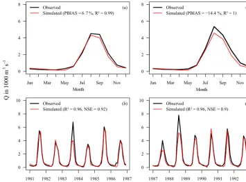
Figure 2 shows the results of monthly and average monthly discharges at gauge El Diem for calibration (left panel) and validation (right panel). According to Moriasi et al. (2007), NSE values of 0.92 (calibration) and 0.90 (validation) are considered to be very good for the monthly time step. The same classification is achieved for the volumetric errors in both periods. The percent bias (PBIAS) between simulated and observed data is−6.7 % (calibration) and−14.4 %

(vali-dation). SWIM simulates peak discharges adequately in most years with few exceptions of rather large underestimation in the years 1983, 1987, and 1988. One explanation for this is the lack of accuracy of WFD inputs and/or observed dis-charge in some years. The simulated amount of water perco-lating into the deep aquifer is about 7 % on average. Without this recharge component, it was not possible to achieve good simulations during the dry period.

Figure S1a and b in the Supplement show the calibration results for the gauges downstream Lake Tana and Kessie. The available GRDC discharge time series for both gauges are rather short and in the case of Tana, the data of the years 1973–1975 are not reliable. Compared to the discharge data given in Dile et al. (2013) and Setegn et al. (2011), maximum discharges are usually around 200–250 m3_s−1_{, as is the case}

in the years 1969–1972 (Fig. S1a). Monthly WFD precipita-tion volumes do not explain the high discharges observed in the last 3 years. Hence, only the first 4 years were used for calibration, where an NSE of 0.67 and a PBIAS of 23.1 % were achieved. Monthly discharges at gauge Kessie in the four years where GRDC data were available are underesti-mated by−18.8 % and achieved an NSE of 0.92. According

(8)

[image:8.612.118.476.83.463.2]

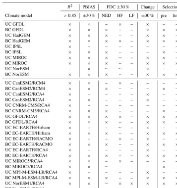
Table 1.Selection of uncorrected (UC) and bias-corrected (BC) Earth system models (ESMs) and regional climate models (RCMs).

R2 PBIAS FDC±30 % Change Selection

Climate model >0.85 ±30 % NED HF LF ±30 % pre final

UC GFDL × × – × – × – –

BC GFDL × × × – – × × ×

UC HadGEM × × × – – × × –

BC HadGEM × × × × – × × ×

UC IPSL × – – – – – – –

BC IPSL × × × – – – × –

UC MIROC × × × ∼ – × × –

BC MIROC × × × – – × × ×

UC NorESM – × ∼ ∼ – × – –

BC NorESM × × × – – × × ×

UC CanESM2/RCM4 × × – × – – – –

BC CanESM2/RCM4 × × × – – – × –

UC CanESM2/RCA4 × – – – – × – –

BC CanESM2/RCA4 × × – – – × – –

UC CNRM-CM5/RCA4 × – – – – – – –

BC CNRM-CM5/RCA4 × × × – – – × –

UC GFDL/RCA4 × × × × – × × ×

BC GFDL/RCA4 × × × – – × × –

UC EC-EARTH/Hirham × – – ∼ – × – –

BC EC-EARTH/Hirham × × × – – × × ×

UC EC-EARTH/RACMO × – – × – × – –

BC EC-EARTH/RACMO × × × – – × × ×

UC EC-EARTH/RCA4 × – – – – × – –

BC EC-EARTH/RCA4 × × × – – × × ×

UC MIROC5/RCA4 × × – × – – – –

BC MIROC5/RCA4 × × ∼ – – – × –

UC MPI-M-ESM-LR/RCA4 × – – – – × – –

BC MPI-M-ESM-LR/RCA4 × × × – – × × ×

UC NorESM1/RCA4 × × ∼ × × × × ×

BC NorESM1/RCA4 × × – – – × – –

“×” is the criterion achieved; “∼” is the criterion almost achieved; “–” is the criterion not achieved. “HF” refers to the high

flows (≤Q₁₀); “LF” refers to the low flows (≥Q₉₀). “Change±30” is the volumetric change between the reference period and

RCP 8.5 in 2030–2059. The abbreviation “pre” refers to the preselection; “final” refers to the models selected in the final ensemble.

to Moriasi et al. (2007) the results for the two gauges can be classified to be between good and very good.

4.2 Model performance

4.2.1 Performance of daily and monthly precipitation

Monthly medians and average annual precipitation sums of UC ESM and RCM simulations deviate sometimes strongly from WFD (see Figs. S2, S3, and S4 in the Supplement). The underlying data for the box plots are monthly precip-itation sums of the 30-year reference period averaged over the UBN catchment area. Bias correction improved the per-formance of both indicators considerably in both model en-sembles. Deviations of average annual precipitation of all BC ESMs are lower than±2 %. The results for the BC RCM

en-semble are more diverse. Five RCMs deviate≤ ±2 %, three

RCMs≤ ±5 %, and two RCMs≤ ±7 %.

Despite the improvement of monthly medians and av-erage annual precipitation sums, bias correction increased the range of monthly precipitation sums critically in sev-eral models in both ensembles. This phenomenon can be ob-served particularly if the deviation of monthly medians be-tween UC simulation and WFD is rather large (e.g. IPSL from May to October, MIROC in July, NorESM in July and August). The effect of increasing variability of monthly pre-cipitation sums is even higher with the method used to bias-correct RCMs and is true for all RCMs (Figs. S3 and S4). The extreme outliers in many models generated by both cor-rection methods are also noticeable.

(9)

pro-0 2 4 6 8

Month

Jan Mar May Jul Sep Nov Observed

Simulated (PBIAS = 6 .7 %, R² = 0.99) (a)

0 2 4 6 8

Month

Jan Mar May Jul Sep Nov Observed

Simulated (PBIAS = −14.4 %, R² = 1) (c)

1981 1982 1983 1984 1985 1986 1987 0

2 4 6 8

10 _Observed

Simulated (R² = 0.96, NSE = 0.92) (b)

1987 1988 1989 1990 1991 1992 1993 0

2 4 6 8

10 _Observed

Simulated (R² = 0.96, NSE = 0.9) (d)

Q

in

1000

m

s

3

Month Month

Year Year

[image:9.612.120.476.66.328.2]

-1

Figure 2.Simulated discharges for calibration(a, b)and validation(c, d)periods at gauge El Diem (Sudan border) using WATCH Forcing Data (WFD). The annual cycle is shown in the top row and average monthly discharges in the bottom row.

nounced in GFDL and MIROC (Fig. S2) and only weakly visible in MIROC/RCA4 (Fig. S4). Although bias correc-tion eliminated this deficiency, it is quescorrec-tionable at what cost. The physical basis was certainly disrupted by the correction method applied.

Tables S3 and S4 in the Supplement show the follow-ing statistical parameters of daily precipitation averaged over the catchment: average number of days with precipitation

>1 mm per annum (nDays>1 mm), average daily

precip-itation (ave), maximum daily precipprecip-itation (max), standard deviation (SD), average precipitation in July, August, and September (ave JAS), and the standard deviation of daily pre-cipitation in July, August, and September (SD JAS). Where Table S3 shows absolute values, Table S4 shows the differ-ences to WFD precipitation (sim-WFD). The two SD param-eters were computed by division, SDsim/SD_WFD. The Tables

show for instance that maximum daily precipitation is under-estimated by all UC models except MIROC. Bias correction resulted in overestimation in 13 out of 15 models. All BC RCMs overestimate maximum daily precipitation, many of them significantly; yet the differences in average daily pre-cipitation of BC simulations are, with exceptions, usually rather small. Large deviations in maximum daily precipita-tion and in the number of rainy days at the same time, while achieving only small differences in average daily precipita-tion, indicate that the distribution of daily rainfall can differ sometimes strongly among simulations. It is also noticeable that the SD of daily precipitation of all UC models is lower

than the WFD SD. Almost all BC simulations show higher SD than the UC simulations, where all ESM SD values are still lower than WFD SD and all RCM SD values are greater than or equal to WFD SD.

4.2.2 Performance of average daily discharge using UC and BC climate input

Bias correction improved the performance of averaged daily discharge simulations (n=365) considerably for all

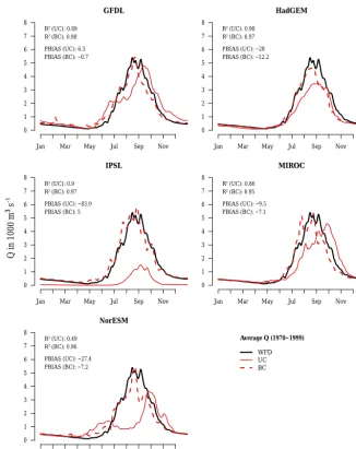
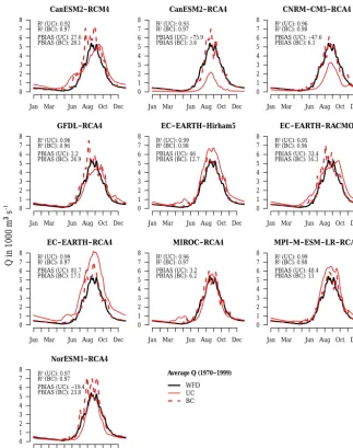
mem-bers of the ESM ensemble and for most memmem-bers of the RCM ensemble. Figures 3 and 4 show the simulated hydrographs in the reference period comparing UC and BC simulations with WFD usingR2and PBIAS to indicate discharge

perfor-mance of the annual cycle.

All UC discharge simulations using ESM climate input, except the one based on GFDL, underestimate average an-nual discharges, which is indicated by negative PBIAS values (Fig. 3). IPSL shows the largest deviations, with a PBIAS of

−84 %. All other models deviate less than 30 % from WFD

discharges.R2 values indicate that seasonal discharge

(10)

[image:10.612.135.462.63.474.2]

Figure 3.Annual cycle of average daily uncorrected (UC) and bias-corrected (BC) simulated discharges at gauge El Diem using Earth system model input and WATCH Forcing Data (WFD) in the reference period (1970–1999).

0.98 but are too low during the high flow season. Another example is the UC IPSL model, which achieves anR2of 0.9,

although it underestimates discharge by−84 %. Hence, high R2values can be misleading if they are not combined with a

volumetric criterion such as PBIAS.

In contrast to ESMs, the majority of discharge simulations based on UC RCMs overestimate average annual discharges in the reference period (Fig. 4). The deviations of six UC RCMs are larger than 30 %. However, seasonal discharge patterns are generally better represented using UC RCM cli-mate input than UC ESM input. The lowest UC RCM R2

value is 0.93 compared to anR2of 0.49 by NorESM of the

UC ESM ensemble. Hence, bias correction improvedR2

val-ues only slightly for 50 % of RCMs. In 60 % of the cases, the volumetric deviation (PBIAS) of BC RCMs is significantly lower than in the corresponding UC models. Based on these

two indicators, the performance of BC RCM simulations is generally better than UC RCMs. However, there is a strong tendency of peak flow overestimation in six out of ten BC RCMs, which is not captured byR2and PBIAS. Therefore,

a visual assessment of hydrographs is important as well as an analysis of daily discharge characteristics using FDCs (see following section).

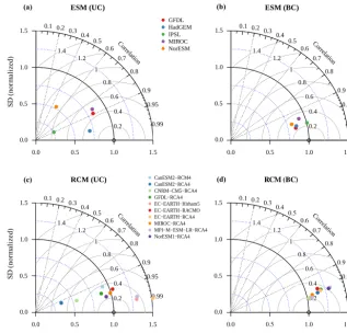
Taylor diagrams (Taylor, 2001) are another method to vi-sualize model performance showing three performance indi-cators (R2, normalized SD, and SDD) in a single plot (see

Fig. 5). They facilitate the visual assessment of model per-formance where outliers can be easily identified. A model with similar statistical characteristics to the reference dataset would be represented by a point at 1.0 on the x-scale and

0.0 on the y-scale. However, interpretation of normalized

(11)

[image:11.612.136.460.65.474.2]

Figure 4.Annual cycle of average daily uncorrected (UC) and bias-corrected (BC) simulated discharges at gauge El Diem using regional climate model input and WATCH Forcing Data (WFD) in the reference period (1970–1999).

Fig. 5a identifies UC IPSL and UC NorESM clearly as out-liers. IPSL is, for instance, an outlier because it shows defi-ciencies at representing SD (0.25 where 1.0 would be ideal) and SDD(0.79 where 0.0 would be ideal). UC NorESM

per-forms poorly in terms of all indicators. After bias correction all ESMs show rather good performance (see Fig. 5b). Except BC IPSL, all models have lower SD than WFD. The charac-teristics of RCMs are different. Half of the UC RCMs’ SDs (Fig. 5c) deviate more than ±0.25 from standardized WFD

but perform much better in terms ofR2. Interestingly, after

bias correction (Fig. 5d), all models show a higher SD than WFD, which is consistent with higher SD of daily rainfall as described in the previous section.

4.2.3 Flow duration curves

(12)

RCM (UC) SD (normalized) SD ( no rm al ize d)

0.0 0.5 1.0 1.5

0.2 0.4 0.6 0.8 1 1.2 1.4 0.1 0.2 _0.3

0.4 0.5 0.6 0.7 0.8 0.9 0.95 0.99 Correl ation ● ● ● ● ● ● ● ● ● ● ● ● ● ● ● ● ● ● ● ●

CanESM2−RCM4 CanESM2−RCA4 CNRM−CM5−RCA4 GFDL−RCA4 EC−EARTH−Hirham5 EC−EARTH−RACMO EC−EARTH−RCA4 MIROC−RCA4 MPI−M−ESM−LR−RCA4 NorESM1−RCA4

ESM (UC) SD ( no rm al iz ed )

0.0 0.5 1.0 1.5

0.2 0.4 0.6 0.8 1 1.2 1.4 0.1 0.2 _0.3

0.4 0.5 0.6 0.7 0.8 0.9 0.95 0.99 Correl ation ● ● ● ● ● ESM (BC)

0.0 0.5 1.0 1.5

0.2 0.4 0.6 0.8 1 1.2 1.4 0.1 0.2 _0.3

0.4 0.5 0.6 0.7 0.8 0.9 0.95 0.99 Correl ation ●● ● ● ● ● ● ● ● ● GFDL HadGEM IPSL MIROC NorESM (a) (b)

(c) (d) RCM (BC)

SD (normalized)

0.0 0.5 1.0 1.5 0.2 0.4 0.6 0.8 1 1.2 1.4 0.1 0.2 0.3_0.4

[image:12.612.139.456.65.369.2]

0.5 0.6 0.7 0.8 0.9 0.95 0.99 Correlation ● ● ● ● ● ● ●● ● ● ● 0.0 0.5 1.0 1.5 0.0 0.5 1.0 1.5 0.0 0.5 1.0 1.5 0.0 0.5 1.0 1.5

Figure 5.Taylor diagram of average daily discharges at gauge El Diem in the reference period (1970–1999). It showsR2, standard deviation

(SD) normalized by SD_ref, and normalized SD_Dof discrepancies for Earth system model (ESM) input in the top row and regional climate model (RCM) input in the bottom row.

high and low flow segments and especially in their extreme values. Note that a logarithmic y-scale is used where large

deviations in the extreme high flow section appear rather small on this plot although they are in fact extremely high.

Figure 6 overcomes this problem by showing relative de-viations of FDCs between discharge time series simulated with climate model inputs and the baseline using WFD. The values corresponding to Fig. 6 are provided by Ta-bles S5–S8 in the Supplement. Assuming that deviations in the range of ±30 % are tolerable, there is not a single UC

model (Fig. 6a and c) which fulfils these requirements for all percentile values. However, the UC ESMs’ MIROC and HadGEM (Fig. 6a) show acceptable deviations (±30 %) in

NED conditions, but there is not a single UC RCM represent-ing NED conditions in the given range (Fig. 6c). The best UC RCM result was achieved with NorESM1-RCA4. Figure 6b and d show that bias correction was successful in correcting the biases of NED for all ESMs and seven out of ten RCMs. The correction method applied to ESMs leads to different patterns in the high and low flow sections compared to the method used to bias-correct RCMs.

Between Q1 and Q10 (high flows), the BC ESMs tend

to underestimate values (but in the given range of accept-able deviations), whereas BC RCMs overestimate flows

cor-responding to these percentiles. There is not a single BC RCM that representsQ₁ conditions in the given range of ±30 %. The smallest overestimation for Q₁ is 52.4 %. All

BC RCMs strongly overestimate extreme high flows Q0.1

andQ0.01. The highestQ0.01 overestimation is 656.9 % and

the lowest 100.4 % (Table S8). The BC ESMs perform bet-ter in the extreme high flow segments. However, only GFDL and HadGEM simulateQ₀.1 values in the acceptable range

and only HadGEM forQ₀.01(Table S6).

In the low flow section (betweenQ₉₀ andQ₉₉) there is

no BC ESM that performs adequately for all percentile val-ues. Except HadGEM that overestimates low flows, the other models tend to underestimate values. Extreme low flows (Q₉₉.9 and Q99.99) are only represented by GFDL within

the acceptable range. The BC RCMs all underestimate low flows, where four models are within the acceptable range of deviations for Q₉₅; there is only one model within this

range forQ₉₉(CanESM2-RCM4). Extreme low flow

condi-tions (Q99.9andQ99.99) are only represented adequately by

EC-EARTH-RCA4; the other RCMs severely underestimate extreme low flows.

(13)

−100 −50 0 50 100

0.01 10 20 30 40 50 60 70 80 90 99 High

flows

Low flows

(a) ESMs (UC)

−100 −50 0 50 100

0.01 10 20 30 40 50 60 70 80 90 99

GFDL HadGEM IPSL

MIROC NorESM

(b) ESMs (BC)

−100 −50 0 50 100

0.01 10 20 30 40 50 60 70 80 90 99 High

flows

Low flows

(c) RCMs (UC)

−100 −50 0 50 100

0.01 10 20 30 40 50 60 70 80 90 99

CanESM2−RCM4 CanESM2−RCA4 CNRM−CM5−RCA4 GFDL−RCA4 EC−EARTH−Hirham5

EC−EARTH−RACMO EC−EARTH−RCA4 MIROC−RCA4 MPI−M−ESM−LR−RCA4 NorESM1−RCA4

(d) RCMs (BC)

% time flow equalled or exceeded % time flow equalled or exceeded

Deviation from baseli

ne [%]

Deviation from baseli

[image:13.612.126.470.64.396.2]

ne [%]

Figure 6.Relative deviations of FDCs from baseline discharge simulation at gauge El Diem using WATCH Forcing Data (WFD) in the reference period (1970–1999). Simulations based on uncorrected (UC) and bias-corrected (BC) Earth system model (ESM) input in the top row and regional climate model (RCM) input in the bottom row.

a few exceptions, both bias correction methods did not im-prove the performance of high and low flows. This is particu-larly true for extreme values, which are strongly exaggerated in most cases.

4.3 Temperature, precipitation, and evapotranspiration projections

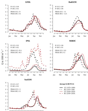
Figures 7, 8, and 9 show precipitation, temperature, and actual evapotranspiration projections of the selected model ensemble (Sect. 4.5) for the 21st century for RCP 4.5 and RCP 8.5 as anomalies to the reference period in the UBN. They indicate the total range of change and the 5-year mov-ing average (MA5) for both scenarios. The precipitation MA5 does not show a distinct trend of change over the cen-tury, but average annual precipitation is projected to be up to 100 mm (∼7 %) higher than in the reference period. The

in-crease is only marginally higher in RCP 8.5 than in RCP 4.5. In Fig. S6 it is shown that a maximum of only three out of 15 UC climate models project decreasing average annual pre-cipitation. The multi-model mean of the CMIP5 ESM ensem-ble projects showed increasing annual precipitation of 5 % in

2030–2059 and 6 % in 2070–2099 under RCP 4.5 and 8.4 % in 2030–2059 and 15.6 % in 2070–2099 under RCP 8.5. Fig-ure S7 shows where the five ESMs used in this study are situated within the entire CMIP5 ensemble. It is noticeable that only three out of 26 ESMs show declining precipitation trends under RCP 8.5.

Projected surface air temperatures show a clearly increas-ing trend over the 21st century in both RCPs. Compared to the reference period, the multi-model mean of the se-lected ensemble projects an increase of 1.7 K (1.5 to 1.9 K) in RCP 4.5 and 2.2 K (1.9 to 3.5 K) in RCP 8.5 in 2050. At the end of the century average temperatures climb up to 2.5 K (1.9 to 4.1 K) under RCP 4.5 and 4.9 K (3.0 to 6.5 K) un-der RCP 8.5. The multi-model mean of the CMIP5 ESM en-semble projects showed increasing average annual tempera-tures of 1.6 K in 2030–2059 and 2.3 K in 2070–2099 under RCP 4.5 and 1.7 K in 2030–2059 and 3.9 K in 2070–2099 under RCP 8.5.

(14)

pe-2020 2040 2060 2080 2100 −500

0 500 1000 1500

Precipitation change in mm

RCP 4.5 RCP 8.5

5−yr moving average Model mean RCP 4.5 Model mean RCP 8.5

[image:14.612.47.287.66.224.2]

Year

Figure 7.Anomalies of annual precipitation amounts relative to the reference period (1970–1999). Range of selected model ensemble.

2020 2040 2060 2080 2100

−2 0 2 4 6 8

Te

m

pe

ra

tu

re

c

ha

ng

e i

n °

C

RCP 4.5

RCP 8.5 5−yr moving averageModel mean RCP 4.5 Model mean RCP 8.5

Year

Figure 8.Anomalies of average annual mean air temperature rela-tive to the reference period (1970–1999). Range of selected model ensemble.

riod. Only in the second half of the 21st century do the pro-jected values increase by up to 50 mm per annum. Hence, it can be concluded that actual evapotranspiration is already at its maximum and can only increase if water availability in-creases too, as is the case after 2050.

4.4 Impact of bias correction on discharge projections Figures 10 and 11 show projected discharge changes of each single model under RCP 8.5 in the period 2030–2059. The changes are relative to the models’ reference period. The fig-ures allow the changes between the reference and the future period of UC and BC models to be investigated, as well as the differences of projected changes between UC and BC simulations. The indicators R2 and PBIAS are not used to

measure the performance, but they indicate the magnitude of change between the reference and the projection period.

The IPSL model shows the largest deviations between the future and the reference period (Fig. 10) for both UC

2020 2040 2060 2080 2100

−300 −200 −100 0 100 200 300 400

E

Ta

c

ha

ng

e i

n m

m

RCP 4.5 RCP 8.5

5−yr moving average Model mean RCP 4.5 Model mean RCP 8.5

[image:14.612.44.289.273.433.2]

Year

Figure 9. Anomalies of annual actual evapotranspiration (ETa) amounts relative to the reference period (1970–1999). Range of se-lected model ensemble.

and BC simulations. The UC IPSL model projects an in-crease of 95.4 % in average annual discharge. A visual as-sessment supports the previously made assumptions that the IPSL model does not provide adequate climate simulations in the study area. This is true for both UC and BC climate simulations. Aich et al. (2014) applied the same five BC ESMs in four large African river basins and found that also in the Niger basin (comparable climate zone to the Blue Nile River) one of the five models projects extreme and unexplain-able changes although it performed adequately in the histor-ical period. In the case of the Niger River basin, it was the MIROC model that behaved awkwardly in the projection pe-riod, whereas the IPSL behaved normally in the range of the other models.

The HadGEM model is the only model where bias correc-tion changed the sign of the discharge signal. The simula-tion with UC climate input projects a decrease of average an-nual discharges of−2.9 % and the BC simulation an increase

of+2.2 %. The results of the NorESM1 model are

interest-ing. The UC model simulates a bimodal rainfall and runoff system with a dry period during the rainy season in July to September. Although the model was forced by bias correc-tion into a completely different system, by pushing the dry season into a rainy season, the projections do not seem any-where near as disrupted as the IPSL simulation. Hence, the NorESM1 results do not support the assumption that strong bias correction necessarily results in unexpected behaviour in future periods. Looking at the change of average peak magni-tudes between UC and BC ESM simulations in the reference and the future period, the change signals are in a similar or-der, except for simulations based on IPSL. They are also in the order of average peaks simulated with WFD input; com-pare with Fig. 3.

(15)

[image:15.612.143.452.65.454.2]

Figure 10.Changes of average daily discharges at gauge El Diem based on uncorrected (UC) and bias-corrected (BC) Earth system model (ESM) input in the period (2030–2059) under RCP 8.5 relative to the models’ reference period (1970–1999). R2and PBIAS values are

computed to show the differences between the projection period and the reference period.

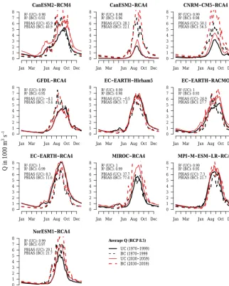
only two UC RCMs simulate higher peaks in the reference period (EC-EARTH-Hirham5 and EC-EARTH-RCA4), five BC RCMs simulate peaks higher than 7000 m3_s−1_{. Looking}

at projected peaks in the period 2030–2059 (RCP 8.5) shows that nine out of ten BC RCM-driven and five UC RCM simu-lations simulate peaks that are higher than 7000 m3s−1_{. The}

projected changes of peak discharge magnitudes between UC and BC RCMs are significantly higher in BC simulations in 50 % of the models. This is not surprising because bias cor-rection of RCMs already led to significant overestimation of high flows in the reference period, as was discussed in Sect. 4.2.3. This behaviour is exaggerated in future periods. 4.5 Selected model ensemble

Table 1 summarizes the performance criteria for all UC and BC simulations usingR2, PBIAS, deviations from FDC

val-ues, and the change rate. The seasonality criterionR2>0.85

was achieved by all simulations except the one based on UC NorESM. Seven out of 30 simulations failed to represent the volumetric deviation criterion PBIAS±30 %.

(16)

[image:16.612.138.461.65.468.2]

Figure 11. Changes of average daily discharges at gauge El Diem based on uncorrected (UC) and bias-corrected (BC) regional climate model (RCM) input in the period (2030–2059) under RCP 8.5 relative to the models’ reference period (1970–1999).R2and PBIAS values

are computed to show the differences between the projection period and the reference period.

model ensemble and is denoted in the column “final”. The latter column indicates that 10 out of 30 simulations passed all performance criteria and thus become members of the se-lected model ensemble. This ensemble consists of four BC ESMs, four BC RCMs, and two UC RCMs.

4.6 Climate impacts on discharges

In this section, the similarities and differences of projected climate change impacts on Blue Nile discharges at gauge El Diem are discussed. The two UC and BC ESM and RCM ensembles and the selected model ensemble are considered (see Table 1, column “final”). In Figs. 12 and 13 and S8–S11, each model simulation is represented by a semi-transparent polygon, where blueish colours indicate an increase and red-dish colours a decrease in monthly discharges. The more

sat-urated the colour, the more models project the same rate of change. The figures show monthly changes relative to aver-age annual discharges in the reference period. This method was chosen in order to avoid overemphasizing large relative changes in dry periods which are not significant compared to annual discharges.

(17)

−4 −2 0 2 4 6

Jan Feb Mar Apr May Jun Jul Aug Sep Oct Nov Dec

4 4 4 2 2 4 1 2 3 5 4 4

1 1 1 3 3 1 4 3 2 0 1 1

Increase in discharge Decrease in discharge

0−n: Number of models projecting pos. or neg. trend

Average annual difference to reference 21.6 % or 41.8 mm (all models) 6.3 % or 13.8 mm (selected models)

(a) ESMs (UC)

−4 −2 0 2 4 6

5 4 4 4 2 2 1 2 5 5 5 5

0 1 1 1 3 3 4 3 0 0 0 0

(b) ESMs (BC)

−4 −2 0 2 4 6

7 7 6 5 5 4 4 6 7 8 8 7

3 3 4 5 5 6 6 4 3 2 2 3

(c) RCMs (UC)

−4 −2 0 2 4 6

7 7 7 7 6 5 4 8 8 8 8 7

3 3 3 3 4 5 6 2 2 2 2 3

(d) RCMs (BC)

Q

c

hang

es

r

el

at

iv

e t

o a

nn

ua

l Q

in

%

Q

cha

ng

es

r

el

at

iv

e t

o a

nn

ua

l Q

in

[image:17.612.98.497.65.372.2]

%

Figure 12.Monthly discharge changes of uncorrected (UC) and bias-corrected (BC) Earth system model (ESM) and regional climate model (RCM) simulations in % under RCP 8.5 (2070–2099). Monthly changes are relative to average annual discharge in the reference period (1970–1999) at gauge El Diem.

Table 2.Projected changes in average annual discharges relative to 1970–1999 in %.

RCP 4.5 RCP 8.5

Model ensemble 2030–2059 2070–2099 2030–2059 2070–2099

UC ESMs 7.4 7.5 8.2 21.6

UC RCMs 18.5 14.2 19.0 12.4

BC ESMs 11.3 20.3 24.5 56.7

BC RCMs 23.5 22.3 27.7 52.7

Selected 5.8 8.4 11.3 13.2

and 56.7 %, and the range of the selected ensemble between 8.4 and 13.2 %. The following conclusions summarize the projected changes of average annual discharges more specif-ically.

– All ensembles in all RCPs and future periods have in common that they all project an increase of average an-nual discharges. An exception is the selected model en-semble of the UC ESMs under RCP 4.5 (2030–2059), which projects a decrease of−0.4 % (Fig. S8a).

– The multi-model means of both UC and BC RCM en-sembles (all models) usually project a higher increase

of average annual discharges than the ESM ensembles, except under RCP 8.5 (2070–2099); see Figs. S9d and S11d.

– The multi-model means of BC simulations (both RCPs and periods) always project higher increases in average annual discharges than the UC multi-model means. – The magnitude of change signals projected by selected

models in the respective ensemble is always lower than the magnitude of the whole ensemble. This is mainly caused by the fact that models projecting changes of

[image:17.612.157.441.451.553.2]

(18)

−4 −2 0 2 4 6

8 7 5 6 4 4 4 4 9 8 8 7

2 3 5 4 6 6 6 6 1 2 2 3

Average annual difference to reference

5.8 % or 16 mm

(a) RCP 4.5 (2030–2059)

−4 −2 0 2 4 6

8 8 8 6 4 3 0 4 9 8 10 9

2 2 2 4 6 7 10 6 1 2 0 1

8.4 % or 23 mm

(b) RCP 4.5 (2070–2099)

−4 −2 0 2 4 6

7 7 6 6 4 5 3 7 8 8 8 9

3 3 4 4 6 5 7 3 2 2 2 1

11.3 % or 30.8 mm

(c) RCP 8.5 (2030–2059)

−4 −2 0 2 4 6

7 6 6 6 3 3 1 5 8 8 8 7

3 4 4 4 7 7 9 5 2 2 2 3

13.2 % or 36.2 mm

(d) RCP 8.5 (2070–2099)

Q

c

ha

ng

es

r

el

at

iv

e t

o a

nn

ua

l Q

in %

Q

c

ha

ng

es

r

el

at

iv

e to a

nn

ua

l Q

in

[image:18.612.113.485.65.349.2]

%

Figure 13.Monthly discharge changes of the selected model ensemble (10 models) relative to average annual discharge in the reference period (1970–1999) at gauge El Diem.

under RCP 8.5, were omitted from the ensemble of se-lected models.

– A noticeable difference between the UC RCM and ESM ensembles is that projected average annual discharges in the far future are lower (RCMs) and higher (ESMs) than in the near future.

There are also general findings concerning changes in sea-sonality.

– There is a trend of decreasing discharges at the end of the dry season projected by all ensembles in both RCPs and periods. The period indicating a drying trend pro-jected by the ESM ensemble tends to be longer and starts a bit earlier (June/July to August) than the trend projected by RCMs (only July).

– There is a trend of increasing discharges during the rainy season projected by all ensembles in both RCPs and periods. The period indicating higher discharges starts earlier in the RCM ensembles (August to ber) than in the ESM ensembles (September to Novem-ber).

– Both ensembles agree that there is almost no change projected in the dry period between December and May.

5 Discussion and conclusions

Are we using the right fuel to drive hydrological models? What are the likely impacts of climate change on future dis-charges in the UBN and is there a strong agreement of pro-jected trends? How far does bias correction influence the re-sults and can we trust models that require strong correction? These questions, posed in the introduction, are discussed in the following.

The majority (≥80 %) of the 15 climate models used in

(19)

may increase by up to 135 % in the same region. Taking the, sometimes contradicting, results of recent studies into account (Teklesadik et al., 2017; Dile et al., 2013; Mengistu and Sorteberg, 2012; McCartney and Menker Girma, 2012; Setegn et al., 2011; Conway and Schipper, 2011; Diro et al., 2011; Elshamy et al., 2009), one can conclude that climate impacts in the UBN are uncertain but there is a bias towards a wetter future. The findings of this study, using the most recent global and regional climate models as well as precip-itation projections of the entire CMIP5 ensemble, underline the latter statement.

Apart from discussing whether the future in the UBN will become generally wetter or drier, decisions with regard to the adaptation of land and water management to changing cli-matic conditions requires not only information on qualitative but also accurate seasonal quantitative changes. The value of using uncorrected climate simulations to answer those ques-tions is, due to the lack of spatio-temporal accuracy and the lack of statistically representative observed weather charac-teristics, usually rather limited. Bias correction of climate simulations is an attempt to overcome at least some of these deficiencies.

The reference dataset used to bias-correct climate models and to calibrate and validate the hydrological model is an-other source of uncertainty. WFD were used in this study be-cause bias correction on ESMs, provided by ISIMIP, was per-formed on the basis of this dataset. Moreover, WFD provide a sound basis as climate input, particularly in data-scarce re-gions, as was shown in various studies (Vetter et al., 2015; Aich et al., 2014; Liersch et al., 2013). The use of a differ-ent reference dataset would certainly require differdiffer-ent cali-bration parameter settings and correction factors but would probably not impact the change signals. The most important issue in this connection is the consistency in using the same reference for calibration, validation, and bias correction.

As was shown in this study, monthly medians and av-erage annual precipitation amounts of UC ESM and RCM simulations deviate sometimes strongly from reference cli-mate. Although bias correction improved the performance of average climate conditions, the range of monthly precip-itation amounts increased critically in several models, pro-ducing some extreme outliers in both ensembles. This phe-nomenon was particularly observed in simulations where de-viations of monthly medians between UC simulations and WFD were rather large in the reference period. Average daily precipitation and the number of rainy days were consider-ably improved by bias correction, but 13 out of 15 BC mod-els overestimate daily precipitation maxima, and many of them significantly. Hence, the bias correction methods ap-plied to ESMs and RCMs in this study could be considered to be only partly successful. While achieving significant im-provement in terms of average daily, monthly, and annual precipitation characteristics, increasing variability of precip-itation amounts, and therefore under- and overestimation of extremes, was the result in many simulations.

This phenomenon is problematic for impact studies and the application of hydrological models, particularly if changes of extreme values are the subject of investiga-tion. Large overestimation of precipitation on some days or in some months, for instance, which are balanced by dry months in the long term, can lead to large amounts of ex-cess water that may be simulated almost entirely as surface runoff by the hydrological model. Therefore, it is reason-able to use hydrological performance indicators to evaluate the suitability of climate simulations, particularly for quan-titative impact studies, and to create a subset of models for the impact assessment. Another way to deal with low perfor-mance in the simulation of extremes in impact studies is to analyse changes in return periods of extreme events (Hatter-mann et al., 2016).

Due to the fact that discharge simulations, based on cli-mate simulations, cannot be compared to observed dis-charges on a real-time daily, monthly, or annual basis, the methods to evaluate discharge performance are limited. In this study, the annual cycle (daily time series averaged over the simulation period) was characterized byR2and PBIAS,

whereR2was a measure of seasonality and PBIAS a

mea-sure of volumetric deviations. Flow duration curves (FDCs) were used to characterize the distribution of average flow conditions, high and low flows, as well as their extremes, by using the whole time series of daily discharge simulations. Unsurprisingly, discharge simulations show similar deficien-cies to precipitation simulations. Using bias-corrected cli-mate simulations improved the performance of non-extreme discharges (NED) significantly but, with few exceptions, the performance of high and low flows did not improve; in fact, it worsened in most of the simulations. Many BC discharge simulations tend to exaggerate high (overestimation) and low flows (underestimation). Comparing peak discharges using UC and BC climate input, for instance, showed a tremendous increase in some BC simulations, although average monthly precipitation patterns of BC models achieved a much bet-ter fit than their UC counbet-terparts. Moreover, the multi-model means of BC simulations (both RCPs and periods) always project higher increases in average annual discharges than the UC multi-model means. However, a hydrological impact study in the Danube River basin showed in turn that relative changes in average monthly discharges projected using UC and BC climate models are overall comparable (Stagl and Hattermann, 2015).