Identification of a change in climate state using regional flood data

Identification of a change in climate state using regional flood

data

Stewart W. Franks

Department of Civil, Surveying and Environmental Engineering, University of Newcastle, Callaghan 2308, New South Wales, Australia

Email: [email protected]

Abstract

Flood frequency analysis typically assumes that annual floods arise from a single distribution and are independent. However, there is significant evidence for the existence of persistent climate modes. Timescales associated with climate variability range from inter-annual through to longer, multi-decadal time scales. In the case of the Australian climate, previous studies of the Indian and Pacific Oceans have indicated marked multi-decadal variability in both mean Sea Surface Temperatures (SST) and typical circulation patterns. In this light, data from 40 stream gauges around New South Wales are examined to determine whether flood frequency data are indeed independent and distributed identically. Given likely correlation in flood records between gauges, an assessment of the regional significance of observed changes in flood frequency is required. To achieve this, flood observations are aggregated into a regional index. A simple non-parametric test is then employed to identify the timing and magnitude of any change in mean annual flood. Finally, it is shown that the identified change in flood frequency corresponds directly to an observed shift in SST and mean circulation. These results demonstrate the role of natural variability in climate parameters and the need for an improved conceptual framework for flood frequency estimation.

Keywords: Floods, flood frequency, climate variability, IPO, PDO, climate change

Introduction

The use of empirical flood frequency analysis is widespread throughout hydrological practice. The basic assumption of flood frequency analysis is that annual maximum flood peaks are distributed independently and identically. The implied assumption is that the climate is statistically ‘static’ at all timescales — the risk of a flood of a given magnitude is taken as being the same from one year to the next, irrespective of the underlying climate mechanisms.

However, it is well known that persistent climate modes modulate regional climates on multiple time scales around the globe. The most well known of such persistent climate modes is perhaps the El Nino/Southern Oscillation (ENSO) operating on an inter-annual time scale. At longer timescales, indices of multi-decadal variability have been derived such as the Pacific Decadal Oscillation (PDO; Mantua et al., 1997) and the Inter-decadal Pacific Oscillation (IPO; Power et al., 1999).

Numerous previous studies have documented regional climate shifts across Australia (e.g. Cornish, 1977; Allan et

al, 1995; Franks and Kiem, 1999; Power et al., 1999). Importantly, there is an abundance of evidence that climate variables affecting Australia shifted significantly during the 1940s. Allan et al. (1995) showed that Indian Ocean Sea Surface Temperatures (SST) were cooler at mid-latitudes and warmer in the subtropical latitudes in the periods 1900 to 1941 when compared with the period 1942 to 1983. In addition they found similar anomalies in surface winds, concluding that the “semi-permanent anticyclone in the mean flow field of the atmosphere over the southern Indian Ocean in the austral summer was weaker in the first 42 years of the 1900s”. Likewise for the Pacific Ocean, Power et al. (1999) demonstrate that the IPO index based on SST (in common with the PDO) displays a strong positive anomaly during the period 1910 to 1945.

anomalies). Similarly, Gershunov and Barnett (1998), and McCabe and Dettinger (1999) have shown how ENSO correlations with American rainfalls vary on multi-decadal timescales. The correlation with ENSO was found to be modulated by long-term PDO persistence in both North Pacific SST data (Mantua et al., 1997) and sea level pressures (Minobe, 1997; 1999). Similar results were obtained in a study of ENSO effects on European rainfalls (Franks, 2000).

Of interest, both IPO and PDO indices are highly correlated (Franks, 2001). A major change in both indices is apparent in the mid-1940s. Despite the observed changes in mid-latitude SST anomalies, exact causal mechanisms have not been proven. Previous studies have raised the prospect that the observed multi-decadal variability in the Pacific might arise from ocean-atmosphere interactions, a response of the ocean to essentially stochastic atmospheric forcing or oscillations between tropical and extra-tropical regions of the ocean (eg. Latif and Barnett, 1994, Gu and Philander, 1997, Minobe, 1999), and even band-specific solar variability (Reid, 1991; 2000; White et al., 1997; Franks, 2001).

Whilst the causal factors for multi-decadal variability remain to be identified, the evidence is growing that regional climate cannot be assumed to be stochastically stationary at these time scales. Given the key role of the oceans in determining general circulation and global weather patterns as well as the variable periods of global warming and cooling observed over the last century, the assumption of stochastic stationarity of climate phenomena, including extremes, cannot be guaranteed. The identification of persistent climate modes suggests that annual maximum floods may not be distributed independently and identically. This study investigates this issue of stationarity.

In the first section of this paper, the Mann-Whitney test for a shift in the mean is applied to data from 40 flood gauges within New South Wales. To identify the most likely year for a transition in flood frequency, the test is applied repeatedly with different trial change years. The typical magnitudes of the identified changes in flood frequency are presented.

The subsequent section attempts to assess the significance of the detected changes through a regionalised approach. To avoid the problem of correlated records providing unwarranted statistical support, a regional index of flood frequency is developed. The analysis is then repeated. The final section of this paper provides a discussion of the results presented and the implications for flood frequency estimation.

Data

The data employed in this study were derived from the PINNEENA data base, developed and managed by the New South Wales Department of Land and Water Conservation. All streamflow records that extend from 1910 onwards were considered. From these gauged records, 40 records spanning 1910 to 1990 were deemed suitable in terms of the length and continuity of record. Figure 1 shows the spatial distribution of the gauged sites within New South Wales. Of these sites, 24 were located in coastal catchments, draining east to the Pacific Ocean, whilst the remaining 16 were in inland catchments belonging to the Murray-Darling basin.

5 . 0 2

1 2 1

2 1 1 1

] 12 / ) 1 (

[

2 / ) 1 (

) ( 1

+ +

+ + −

=

∑

N N N N

N N N y R Z

N

t t

c

Step change detection

To detect a step change in the individual flood time series, the simple Mann-Whitney test is employed. This test assesses the difference in the means of two sub-series arising from splitting of the complete series. It is important to note that the test is non-parametric thereby avoiding the need to manipulate the flood data to approximate any pre-conceived distribution.

To perform the test, a time series of annual maximum flood data, y_t, t = 1, …, N, is broken into two sub-series, y₁, …, y_N1 and y_N1+1, …, y_N2 of sizes N₁ and N₂ respectively. The original time series is then rearranged in increasing order of magnitude to produce the new series, z_t, t = 1, …, N. The test of the hypothesis that the mean of the first sub-series is equal to the mean of the second sub-series is then achieved through calculating the Mann-Whitney test statistic;

(1) Fig. 1. Location of gauged sites used in study (New South Wales,

where R(y) is the rank of observation y_t in ordered series z_t (Salas, 1993). The hypothesis of equal means is rejected if |Z_c| > Z_(1-a/2), where Z_(1-a/2) is the (1-a/2) quantile of the normal distribution. In the context of the present study, the application of this test assumes that two distinct ‘climate states’ are evident in the flood records.

Results – Analysis of individual flood

gauges

The Mann-Whitney test (Eqn. 1) was applied to each of the 40 flood gauges independently. Treating the year of transition of climate state (N₁) as an unknown, the test was applied repeatedly, with N₁ ranging from 1920 through to 1970. For each gauge, the trial year that returned the highest Z statistic was selected as the optimum year of transition. The methodology is then repeated for each gauge.

Figure 2 shows a histogram of the identified optimum transition years for those gauges with differences in the mean flood significant at the 99% level. As can be seen, the analysis of the individual gauges shows marked consistency in that the identified transition years are primarily in the 1940s. Note that this is in strong agreement with the observed changes in regional sea-surface temperature and circulation patterns identified by Allan et al., (1995). It is also worth noting that 19 of the 40 (48%) gauges show 99% significant differences, 16 of these during the 1940s.

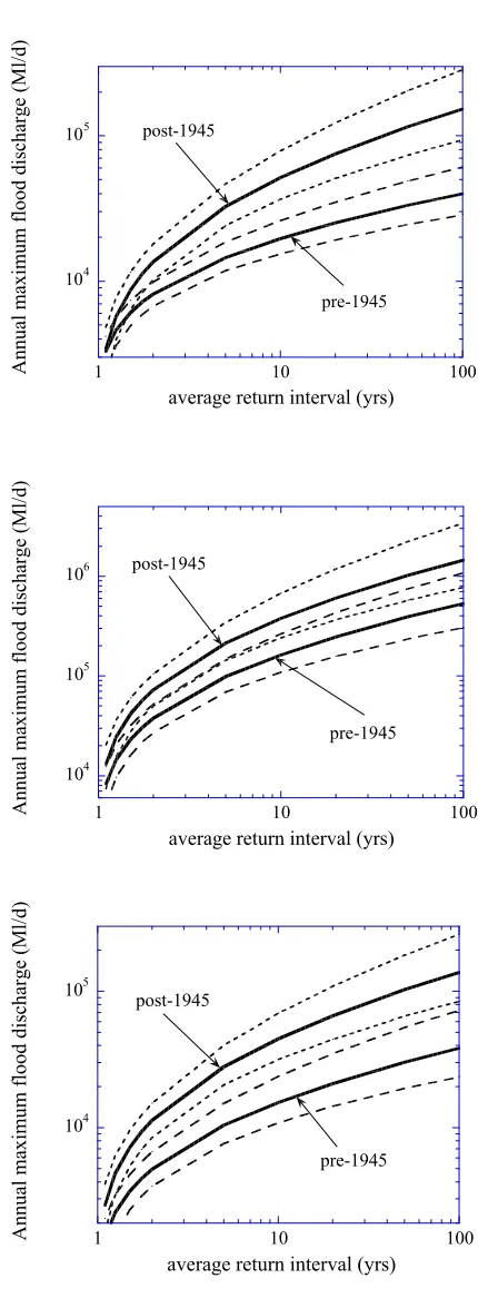
To demonstrate the degree of change in the flood frequency distributions, three of the records from these gauges were selected and stratified at 1945 and log-normal frequency curves were fitted. Figure 3shows the resultant curves and 90% probability intervals for the pre- and

post-1945 stratification. As can be seen, differences in the frequency distributions are marked.

Whilst the results in Figs. 2 and 3 do indicate a marked change in flood characteristics around the early 1940s, it is

0 1 2 3 4 5 6 7

1920 1930 1940 1950 1960 1970

Count

Optimum transition year

Fig. 2. Histogram of the optimum transition years for those gauges returning differences significant at the 99% level.

Fig. 3. Log-normal expected quantiles and their 90% probability limits (dashed lines) for three sites in study region, stratified at 1945.

104 105

1 10 100

Annual maximum flood discharge (Ml/d)

average return interval (yrs)

pre-1945 post-1945

104 105 106

1 10 100

Annual maximum flood discharge (Ml/d)

average return interval (yrs)

pre-1945 post-1945

104 105

1 10 100

Annual maximum flood discharge (Ml/d)

average return interval (yrs)

post-1945

also possible that the results reflect a sampling error of highly correlated gauges. To address this, the following section derives an index of regional flood characteristics.

Derivation of regional indices

The results presented in the previous section are highly suggestive of a marked step change in flood frequency taking place around the mid-1940s. As noted earlier, Cornish (1977) demonstrated a similar step change in annual rainfall during the mid-1940s, providing corroborative evidence that the observed change in flood frequency is not due to any undocumented ‘nuisance’ factor (for example, gauge design, instrumentation, etc.). Of additional importance, the inferred change corresponds well to analyses of changes in regional SST and circulation patterns, providing further evidence of an external climatological causal factor (Allan et al., 1995; Power et al., 1999). However, whilst the inferred change is marked, the methodology employed seeks to maximise this difference. It may therefore be suspected that the 40 gauges are highly correlated. The increase in flood frequency may arise from a simple sampling error and the timing of the transition in flood frequency, corresponding to observed changes in external forcing variables (SST and circulation) and annual rainfall, may be merely coincidental. Whilst this seems highly unlikely, this can nonetheless be tested through an analysis of a regional index of flood frequency.

If the flood gauges were correlated perfectly, treating them as entirely uncorrelated would imply 40 independent records with any inferred change having substantial statistical support. In fact, if the gauges were correlated perfectly the true support would be equivalent to that of a single record. Developing a regional index of flooding, in effect collapses the flood data into a single time series, with any correlation between gauges being accounted for implicitly. Adopting this alternative extreme, if the gauges are not perfectly correlated (as would seem most likely), the statistical support of the 40 gauges, if anything, was under-estimated. This simplified approach is adopted here.

In this study, a regional index is derived through a purely statistical approach — the individual records are scaled by the mean of the log annual flood maximum discharge. The log is used in this study to weight each gauge equally under the assumption of a log-normal flood frequency model. For example;

(2)

where x_tj _{is the normalised index for gauge, j, at time, t, and}

where N is the total length of the flood record. For each

year, the resultant 40 scaled time series are then averaged to provide a gauge-mean log maximum;

for t = 1, …, N (3)

where RI_t is the normalised regional index, and M is the total number of gauges. The advantage of this approach is that each gauge is weighted equally in the derivation of the regional index as a function of the typical magnitude of the annual flood.

Results – Analysis of regional index

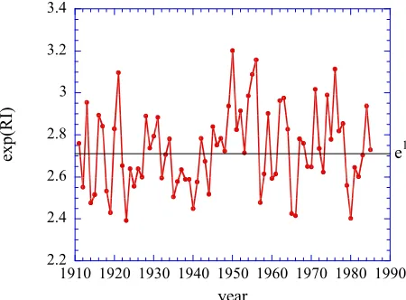
The regional index was derived as described above. Figure 4 shows the resultant time series. The Mann-Whitney test was then applied repeatedly to the time series, with trial values of the transition year, N₁, ranging from 1920 to 1970. Figure 5 shows the calculated Z_c statistics for each of the

∑

= N

i j i

j t j

t

N Q

Q x

1

/ ln ln

M

x

RI

j j t

t

/

1

∑

=

2.2 2.4 2.6 2.8 3 3.2 3.4

1910 1920 1930 1940 1950 1960 1970 1980 1990

exp(RI)

year

e1

0.0 0.5 1.0 1.5 2.0 2.5 3.0

1910 1920 1930 1940 1950 1960 1970 1980 year

|Z c

| statistic

99%

95%

Fig. 4. Time series of the derived regional index

Fig. 5. Calculated |Z_c| statistic for the different trial transition years using the regional index. Note the sharp peak at 1944, significant at

different trial transition years. As can be seen, the derived index shows that the most likely transition year is 1944, again in strong accordance with the observed changes in SST and circulation patterns (Allan et al., 1995; Power et al., 1999) and annual rainfall (Cornish, 1977). The optimum Z_c statistic for the index is 2.65, indicating a statistical significance greater than 99%.

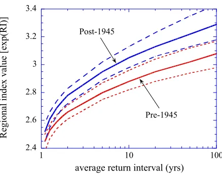
Finally, Fig. 6 shows the resultant growth curves and the 90% quantiles of the derived regional index, stratified at 1945 (N₁+1). As can be seen clearly, the probability limits do not overlap, indicating that the difference between the stratified samples is not due to sampling uncertainty and that the significance of the difference is greater than 99% (e.g. > 1 – [0.05*0.05]). This, in tandem with the known change in climate variables in the mid-1940s, provides irrefutable evidence that the flood frequency distributions, pre- and post-1945, are not identical.

Conclusions

This paper has sought to test the assumption of flood events as independent and identically distributed events. The results demonstrate unequivocally that, for New South Wales, the assumptions of empirical flood frequency analysis do not hold. Two distinct periods of different flood risk are markedly apparent in the flood data. Prior to 1945, floods of high magnitude are not present in the records. After 1945, flood risk increased dramatically. The observation of a marked change in flood risk around 1945 corresponds strongly to the observed changes in Indian and Pacific Ocean sea-surface temperatures and regional circulation patterns around Australia (Allan et al., 1995; Power et al., 1999). This provides strong external evidence that multi-decadal Fig. 6. Log-normal expected quantiles and their 90% probability limits (dashed lines) for three sites in the study region, stratified at

1945 (N₁+1 = N₂). 2.4

2.6 2.8 3 3.2 3.4

1 10 100

Regional index value [exp(RI)]

average return interval (yrs)

Pre-1945 Post-1945

climate processes may, in many instances, invalidate the assumptions of a purely empirically-based flood frequency analysis.

One of the key implications of this result is that flood frequency analysis performed without knowledge of the climate state from which the data are drawn may lead to gross under- or over-estimation of the true long-term flood risk. In the case of New South Wales, if data prior to 1945 are used, the long-term flood risk will be underestimated. If data after 1945 are employed, the true long-term risk may be over-estimated. It is therefore clear that a more thoughtful approach to estimating flood risk is required — flood data must be assessed as a function of the causal climatological factors (or climate states) that affect regional climates.

Whilst this study has focused on New South Wales, it must be expected that substantial variability is also present in many other parts of the globe. As noted earlier, persistent climate modes of multi-decadal time scales have been identified and shown to influence markedly regional climates around the globe (e.g. Mantua et al., 1997; Keily, 1999; Landman and Mason, 1999; Nigam et al., 1999). It is therefore apparent that empirical hydrological analyses must be adapted to account for any secular variability identified as a result of changing climatological factors. This will necessitate a strong multi-disciplinary approach.

Finally, the results presented here are also of importance in the assessment of the role of anthropogenic influences on climate. The changes observed are unlikely to be related to increased atmospheric concentrations of radiatively-active gases as concentrations have begun to increase only recently (1970s onwards) in a substantially exponential manner. More likely, the observed step change may be just one manifestation of natural climate variability. It is clear that natural variability is a key factor of the Australian climate and must be fully understood before an objective analysis of the risks of anthropogenic climate change can be achieved.

Acknowledgements

This study was funded by the Australian Research Council SPIRT scheme, with collaborative industry funding from Hunter Water Corporation, and with additional funds provided by the Royal Society of Edinburgh. This paper was improved through the comments from Jim McCulloch and two anonymous reviewers.

References

Cornish, P.M., 1977. Changes in seasonal and annual rainfall in New South Wales. Search, 8, 38–40.

Franks, S.W., 2000. On the variable influence of ENSO on European rainfalls, Research Report No. 191.2000, University of Newcastle, Australia, 30pp.

Franks, S.W., 2002. Assessing hydrological change: deterministic GCMs or suprious solar correlation? Hydrol. Process., 16, 559– 564.

Franks, S.W. and Kiem, A.S., 1999. Inter-decadal variability of rainfall at selected sites across coastal New South Wales. Proceed. ICB-ICUC, Sydney, Australia, Nov. 1999. On CD issued by Macquarie University, Sydney, ISBN: 1 86408 543 6 Gershunov, A. and Barnett, T.P. 1998. Interdecadal modulation of ENSO teleconnections. Bull. Amer. Meterol. Soc., 79, 2715– 2726.

Gu, D.F. and Philander, S.G.H, 1997. Interdecadal climate fluctuations that depend on exchanges between the tropics and extratropics. Science, 275, 805–807.

Keily, G., 1999. Climate changes in Ireland from precipitation and streamflow observations. Adv. Water Resour., 23, 141–151. Landman, W.A. and Mason, S.J., 1999. Change in the association between Indian Ocean sea-surface temperatures and summer rainfall over South Africa and Namibia. Int. J. Climatol., 19, 1477–1492.

Latif, M. and Barnett, T.P., 1994. Causes of decadal climate variability over the North Pacific and North America. Science, 266, 634–637.

Mantua, N.J., Hare, S.R., Zhang, Y., Wallace, J.M. and Francis, R.C., 1997. A Pacific decadal climate oscillation with impacts on salmon. Bull. Amer. Meteorol. Soc., 78, 1069–1079.

McCabe, G.J. and Dettinger, M.D., 1999. Decadal variations in the strength of ENSO teleconnections with precipitation in the western United States. Int. J. Climatol., 19, 1399–1410. Minobe, S., 1997. A 50–70 year climatic oscillation over the North

Pacific and North America. Geophys. Res. Lett., 24, 683–686. Minobe, S., 1999. Resonance in bidecadal and pantadecadal climate oscillation over the North Pacific: Role in regional climate shifts. Geophys. Res. Lett., 26, 855–858.

Nigam, S., Barlow, M. and Berbery, E.H. 1999. Analysis links Pacific Decadal variability to drought and streamflow in the United States. EOS, Trans. Amer. Geophys. Union, 80, Dec 21 1999.

Power, S., Casey, T., Folland, C., Colman, A. and Mehta, V., 1999. Inter-decadal modulation of the impact of ENSO on Australia. Clim. Dynamics, 15, 319–324.

Reid, G.C., 1991. Solar total irradiance variations and the global sea surface temperature record. J. Geophys. Res., 96, 2835– 2844.

Reid, G.C., 2000. Solar variability and the Earth’s climate: Introduction and overview. Space Sci. Rev., 94, 1–11. Salas, J.D., 1993. Analysis and modeling of hydrologic time series,

In: Handbook of Hydrology, D.R. Maidment (Ed.), 19.1–19.72, McGraw-Hill, New York.