Performance analysis of different array configurations for smart antenna applications using firefly algorithm

PERFORMANCE ANALYSIS OF DIFFERENT ARRAY CONFIGURATIONS

FOR SMART ANTENNA APPLICATIONS USING FIREFLY ALGORITHM

K. Sridevi

and A. Jhansi Rani

Research Scholar, ECE Department, ANU College Of Engineering, Acharya Nagarjuna University, Guntur, Andhra Pradesh, India 2_{ECE Department, VR Siddhartha Engineering College, Vijayawada, Andhra Pradesh, India}

Email: [email protected]

ABSTRACT

Voluminous studies have already been conducted on smart antennas. Mostly these studies dedicated to Uniform linear array, Rectangular array and circular array configurations. This paper aims at the investigation of the beam forming capabilities of uniform hexagonal array (UHA) and planar uniform hexagonal array (PUHA) configurations as compared to circular array by controlling amplitude excitation only using firefly algorithm. Results are compared with that of particle swarm optimization technique. Comparisons are made in the context of adaptive beam forming capabilities of the three array configurations.

Keywords: uniform hexagonal array, particle swarm optimization, smart antennas.

1. INTRODUCTION

Smart antennas are able to bring excellent capacity improvement to the frequency resources confined to radio communication systems by proficient frequency reuse scheme. This unique feature has been made profitable through remarkable advances in the digital signal processing field which enable smart antennas to nullify the interferences while focusing on predetermined user dynamically.

The capacity of a radio communication channel can be improved by MIMO-SDMA technique. This technique allows multiple signals to share a co channel at the same time. Therefore, these signals will interfere with one another. The uplink MIMO-SDMA technique allows the allotment of multiple users to a common communication channel with its ability of spatial separation and nullifying the interferences, thereby system capacity can be improved. Smart antenna system draws more attention in mobile communication as it is able to place nulls to prevent co channel interferences and steer the main lobes of radiation pattern towards the intended users [1].

There are different null steering methods which include controlling of amplitude only, phase only, the position only and the complex weights that control both amplitude and phase of the array elements. Out of all methods null steering with complex weights is efficient but is expensive since each array element requires phase shifters and variable attenuators where as the amplitude-only control [2] uses amplitude-only variable attenuators to adjust the element amplitudes and also the computational time and number of elements becomes halved if the element amplitude possess even symmetry where as computational time increases as the number of array elements increased for complex weights. The phase- only control uses phase shifters while position-only control uses mechanical

Most of the research work has been done on the analysis of smart antennas which primarily involves the study of uniform linear, rectangular and circular array configurations. In this paper, analysis of two different array configurations such as uniform hexagonal array (UHA) and planar uniform hexagonal array (PUHA) has been carried out and compared with circular array configuration by using Fire fly algorithm which outperforms the particle swarm optimization.

2. DIFFERENT ARRAY GEOMETRIES

In this paper, three different array configurations circular, hexagonal and planar hexagonal array are considered in which isotropic elements are distributed uniformly. Firefly algorithm is employed to obtain optimum weights that maintain deep nulls. We compare the three array configurations in the context of adaptive beam forming capability [3].

2.1 Circular array

The geometry shown in Figure-1 is circular antenna array of radius r and consists of isotropic sources of N elements that are uniformly distributed. Let the circular array is laid on the x-y plane (∅ = 900) with its centre is at the x-y plane origin. The array factor is given by

𝐴𝐹(∅, 𝜃) = ∑𝑁𝑛=1𝐴𝑛 𝑒𝑗𝑘𝑟 sin ∅(cos 𝜃𝑛cos 𝜃+sin 𝜃𝑛sin 𝜃) (1)

Where 𝐴_𝑛 relative amplitude of nth element is, 𝜃 is azimuthal angle from positive x-axis to the observation point, ∅ is the elevation angle from positive Y-axis to the observation point. 𝜃_𝑛 is the angle between positive x-axis to nth element and it is given by the equation

Figure 1. Circular array of 12 elements are uniformly distributed

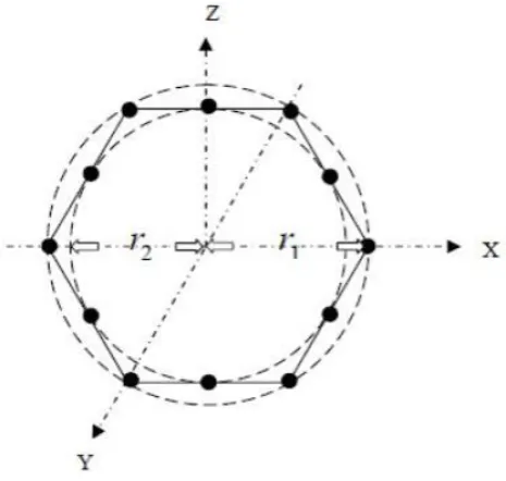
2.2 Hexagonal array

The Figure-2 shows hexagonal array [4] and can be treated as it consists of two N-elements of concentric circular arrays of two distinct radii r1 and r2. There are a total of 2N elements out of which N elements are placed at the vertices and the other N elements are placed at mid points of the sides of hexagon. The array factor of the hexagonal array is given by

𝐴𝐹(∅, 𝜃) = ∑𝑛𝑛=1[𝐴𝑛𝑒𝑗𝑘𝑟1sin 𝜃(cos ∅1𝑛cos ∅+sin ∅1𝑛sin ∅) +

𝐵𝑛𝑒𝑗𝑘𝑟2sin 𝜃(cos ∅1𝑛cos ∅+sin ∅1𝑛sin ∅) ] (2)

Where 𝐴_𝑛 and 𝐵_𝑛 are relative amplitude excitations of N- elements placed at the vertices aid points of the hexagon respectively. 𝑟₁ and 𝑟₂ given as

𝑟1=_sin(𝑑𝜋 𝑁)

, and 𝑟₂= 𝑟₁cos (𝜋

𝑁) in which d is the inter element spacing along any side of hexagonal array and ∅1𝑛 and ∅2𝑛 respectively are angles between positive x-axis and nth element at vertices and midpoint of the hexagon.

Figure-2. Hexagonal array of 12 elements arranged in two concentric circular rings.

2.3 Planar uniform hexagonal array

Two concentric hexagonal arrays are arranged as shown in Figure-3. There are 2N elements are arranged in equal number on the two concentric hexagonal arrays [5]. The array factor of planar uniform hexagonal array is given by equation

𝐴𝐹(𝜃, 𝛷) =

∑𝑀𝑚=1∑𝑁𝑛=1{[𝐴𝑛𝑚𝑒𝑗𝑘𝑟1𝑚sin 𝜃(cos ∅1𝑛cos ∅+sin ∅1𝑛sin ∅) +

𝐵𝑛𝑚𝑒𝑗𝑘𝑟2sin 𝜃(cos ∅2𝑛cos ∅+sin ∅2𝑛sin ∅)]} (3)

Where 2N is number of elements on each hexagon, M is the number of concentric hexagons and d is spacing between two hexagons.

𝑟1𝑚=_sin(𝑑𝜋 𝑁)

and 𝑟_2𝑚= 𝑟_1𝑚cos (𝜋 𝑁)

For maximizing the out power in the intended signal direction at 𝛷_𝑖 and in the interferers direction at 𝛷_𝑗, to minimize the total output power, the following objective function [5] is used.

Figure-3. Planar uniform hexagonal array of 12 elements are arranged on two concentric hexagonal rings.

3. FIRE FLY ALGORITHM

Firefly algorithm was based on the behavior and flashing patterns of fireflies. It was developed by Xin-She-Yang in 2008. Essentially Firefly algorithm follows three idealized rules which were mentioned in [9]. The

attractiveness is denoted as β that each firefly has and is

described by invariably decreasing function of the distance 'r' between any two fireflies.

𝛽(𝑟) = 𝛽0𝑒−ϒ𝑟𝑚 for 𝑚 ≥ 1

Where 𝛽₀ represents the maximum attractiveness at r=0 and the factor ϒ which controls the decrease of the light intensity is called light absorption coefficient.

If the positions of two fireflies m and n are denoted as 𝑥_𝑚 and 𝑥_𝑛, then the distance between two fireflies m and n is given as

𝑟𝑚𝑛 = ‖𝑥𝑚− 𝑥𝑛‖ = √∑ (𝑥𝑑𝑘=1 𝑚,𝑘− 𝑥𝑛,𝑘)2 (5)

Where 𝑥_𝑚,𝑘 is the kth component of spatial coordinate 𝑥_𝑚 of the mth firefly and d signifies the dimension number. The mth firefly movement can be determined from the following equation

𝑥𝑚= 𝑥𝑚+ 𝛽0𝑒−ϒ𝑟2𝑚,𝑛(𝑥𝑚−𝑥𝑛)+ 𝛼 (𝑟𝑎𝑛𝑑 −1₂) (6)

in which the first term represents mth firefly current position, second term signifies attractiveness of a firefly and the last term is used for the arbiter movement if there is no brighter firefly. 𝑟𝑎𝑛𝑑 is an arbitrary number that is uniformly distributed in the range 0 and 1. For most of the

cases α is in the range between 0 and 1 and 𝛽0=1. The characteristic length is denoted as Г= ϒ−1𝑚

for fixed ϒ and also Г→ 1 as 𝑚 →∞. Two important limiting cases when ϒ → 0 and ϒ →∞. When ϒ → 0, the

attractiveness β becomes 𝛽0 and Г→∞,from which we can say that there is no decrease of light intensity. Thus anywhere in the domain, a glowing firefly can be seen. Thus, a global optimum can be reached easily. When ϒ →∞ on the other hand, leads to Г→ 0 and 𝛽(𝑟) → 𝛿(𝑟) which is a Dirac delta function means that fireflies are short sighted as attractiveness is almost zero. No other fireflies can be seen and each firefly moves completely in random fashion. This corresponds to random search method completely. It is possible to tune the parameter ϒ

and α that it can be better than random search and Particle

Swarm Optimization (PSO). FA can find simultaneously both global optima and local optima [10].

4. SIMULATION RESULTS

Different shapes of array geometries are considered and compared with each other. The first array considered is a UCA with 12 isotropic elements uniformly distributed with a radius of 7.6

2𝜋λ. Also hexagonal array of inner radius r1 is 3.6

2𝜋𝜆 and outer ring radius r2 is 4

Figure-4. Radiation pattern of PUHA when SOI is 00 and SNOI is 650 and -650 using PSO and Firefly algorithms.

-80 -60 -40 -20 0 20 40 60 80

-90 -80 -70 -60 -50 -40 -30 -20 -10 0

theta(in degrees)

A

rr

a

y

f

a

c

to

r

(A

F

)i

n

D

b

PSO Firefly

10 20 30 40 50 60 70

C

o

s

t

Best Cost vs Iteration

Figure-6. Radiation pattern of of the three array configurations for SOI is 00 and SNOI is 650 And -650 using PSO algorithm.

Figures 6 and Figure-7 shows the radiation patterns of circular, hexagonal and planar hexagonal array using PSO and firefly algorithm respectively. A first observation from these plots is that as compared to other two geometries, PUHA achieves the deepest nulls towards the interference direction. Especially with Firefly algorithm, the nulls with PUHA towards the interferers are

very deep which a desirable property is. PUHA also gives narrowest main beam widths. UHA gives more null depth than UCA and UCA gives more side lobes as compared with UHA [6]. PUHA achieves highest directivity as the main beam width is narrow. The respective beam widths and null depths are tabulated in Table-1 and Table-2 using PSO and Firefly algorithms.

Table-1. Beam width and null depth comparison of circular, hexagonal and PUHA using PSO.

Parameter Circular Hexagonal PUHA

1. Null depth (in dB)

-46.01 -56.7 -60.6

2. Beam width

(in degree) -25 -25 -10.6

-80 -60 -40 -20 0 20 40 60 80

-90 -80 -70 -60 -50 -40 -30 -20 -10 0

theta(in degrees)

A

rr

a

y

f

a

c

to

r

(A

F

)i

n

D

b

Figure-7. Radiation pattern of of three array configurations for SOI is 00 and SNOI is 650 and -650 using firefly algorithm.

Table-2. Beam width and null depth comparison of circular, hexagonal and PUHA using Firefly algorithm.

Parameter Circular Hexagonal PUHA

1. Null depth (in dB) -60 -55 -62

2. Beam width (in degree) -24.2 -24.2 -10.8

5. CONCLUSIONS

In this paper, smart adaptive arrays such as UCA, UHA and PUHA are considered and the main issue related to smart antennas, adaptive beam forming was investigated for all arrays with the same number of elements by using Particle Swarm Optimization and Firefly algorithm. The investigation reveals that Hexagonal array geometry gives slightly deeper nulls as compared to circular array with the same beam width also it is smaller overall size. PUHA achieved the deepest nulls towards the angles of interference, especially when

[2] K. Guney. 2008. Interference suppression of linear antenna arrays by amplitude only control using a Bacterial Foraging Algorithm. Progress in Electro magnetics Research. 79: 475-497.

[3] Ioannides P. and C. A. Balanis. 2005. Uniform circular and rectangular arrays for adaptive beamforming applications. IEEE Antennas and Wireless Propagation Letters. 4: 351-354.

-80 -60 -40 -20 0 20 40 60 80

-90 -80 -70 -60 -50 -40 -30 -20 -10 0

theta(in degrees)

A

rr

a

y

f

a

c

to

r

(A

F

)i

n

D

b

Algorithm. Progress in Electro magnetics Research. 72: 75-90.

[6] Gozasht F., G. R. Dadashzadeh and S. Nikmehr. 2007. A comprehensive performance study of circular and hexagonal array geometries in the LMS algorithm for smart antenna applications. Progress in Electromagnetics Research, PIER.68, 281-296.

[7] Chen T. B., Y.B. Chen, Y. C. Jiao and F. S. Zhang. 2005. Synthesis of antenna array using particle swarm optimization. Microwave Conference Proceedings, 2005. APMC 2005. Asia-Pacific Conference Proceedings.

[8] Yang X.-S. 2010. Firefly algorithm, stochastic test functions and design optimization. International Journal of Bio-inspired Computation. 2(2): 78-84