Statistical Analysis of Climate Factors Influencing Dengue Incidences in Colombo, Sri Lanka: Poisson and Negative Binomial Regression Approach

ISSN 2250-3153

Statistical Analysis of Climate Factors Influencing

Dengue Incidences in Colombo, Sri Lanka: Poisson and

Negative Binomial Regression Approach

Leslie Chandrakantha

Department of Mathematics and Computer Science, John Jay College of City University of New York, New York, USA

DOI: 10.29322/IJSRP.9.02.2019.p8616 http://dx.doi.org/10.29322/IJSRP.9.02.2019.p8616

Abstract- Dengue fever is a mosquito–borne disease caused by the dengue virus. Transmission of the virus depends on the presence of Aedes mosquito. Dengue has become a global problem and is common in more than a hundred countries. It is most prevalent in tropical and subtropical regions. It has been a major public health challenge in Sri Lanka in recent years. Mosquito generation and the spread of dengue are known to be influenced by the climate. Identifying the climate factors that affect dengue outbreaks would be helpful to take necessary actions to prevent the spread of dengue. In this paper, we study the climate factors affecting the spread of dengue in the city of Colombo, Sri Lanka from the period of 2010 to 2018. The Poisson and negative binomial regression models were employed to analyze the data. These models fit the monthly dengue incidences against the temperature, rainfall, and relative humidity. This study showed a significant association between monthly dengue incidence and the amount of rainfall. The negative binomial model fits the data more accurately due to the nature of overdispersed data. This study provides useful information in predicting dengue incidences and developing a future warning system.

Index Terms- Dengue Incidences, Negative Binomial Regression, Overdispersion, Poisson Regression, Rainfall,

I. INTRODUCTION

engue fever is a viral disease and it is the most common mosquito-transmitted disease among humans on a world-wide basis. As many as 400 million people are infected annually [1]. Dengue has emerged as a worldwide problem since the 1950s. Typically, the symptoms of dengue fever are similar to those of the flu. In some cases, the patient will develop a lack of blood platelets which, in turn, may develop into a dangerous condition if left untreated. There are not yet any vaccines to prevent infection with the virus and the most effective protective measures are those that avoid mosquito bites.

Sri Lanka is one of the leading countries affected from dengue in recent years. Dengue infections have been endemics in Sri Lanka since the mid-1960s. Dengue fever was serologically confirmed in Sri Lanka in 1962 [2]. The prevalence of dengue infections on a yearly basis has been increasing over time. Now it has become the leading killer mosquito infection in Sri Lanka [3]. In urban areas, the disease incidence is the highest, especially in Colombo district, the most densely populated part of the country. According to the Sri Lankan Epidemiology Unit of Health Ministry [4], 399,262 incidences of dengue fever have been reported in last six years including 2018. Out of these, 96,677 incidences came from Colombo district which is among 25 districts of the country. The Colombo District dengue incidences are about 24% of the total incidences reported in the country. Colombo District is subdivided in two parts, namely, Colombo city area (Colombo Municipal Council) which is the capital of the country and out of Colombo Municipal Council area. Colombo District has 270 square miles (699 square kilometers) of total land area in which 14 square miles (27 square kilometers) of area belong to Colombo city. Data from epidemiology unit shows that nearly 25% of the dengue incidences in Colombo District came from Colombo city in last 6 years. Based on these data, the population of the city, and the importance of location of the Colombo in the country, we focus our study of dengue incidence on Colombo City.

ISSN 2250-3153

climate data. Kavinga et al. [7] proposed a model to predict dengue disease outbreaks using a vector correction method. Their model was based on the humidity and temperature. They have noted that their model approximately provides reliable predictions. Sun et al. [8] stated that the differences on the effects of weather on dengue incidences could be due to the different variations of the amount of rainfall or the range of temperatures in different regions with respect to their geographical locations. Their findings were based on the analysis of spatial-temporal distribution of dengue in Sri Lanka from 2012 to 2016. Karim at el. [9] developed a prediction model using multiple linear regression for dengue incidences in Dhaka, Bangladesh. They have noted that their model had some limitations in predicting the monthly number of dengue incidences. Hii at el. [10] used piecewise linear functions to develop a time series model to predict dengue incidences and to provide an early warning in Singapore. Their model forecasted dengue incidences up to 16 weeks ahead using retrospective weekly mean temperature and cumulative rainfall. Iguchi at el. [11] used the wavelet coherence analysis to determine the presence of non-stationary relationships between meteorological variables and dengue incidences in Philippines. Their finding indicated that meteorological variables have varying effects on dengue incidences.

As we indicated above, the impact of climate factors on dengue incidence rates has attracted considerable attention in recent years. The role of climate as a driving force for infection is still a subject of considerable attention. Temperature affects the development rates and survival of mosquito vectors while rainfall influences the availability of mosquito larvae habitats and breeding grounds for mosquitos. High levels of relative humidity are known to increase the lifespan of mosquitos [12].

These three climate factors may have synergistic effect on dengue transmission.

In this paper, the association between dengue incidence and climate variables are modeled using Poisson and negative binomial regression models. The Poisson and negative binomial regression are commonly used for modeling the number of events (counts) occurring within a certain time interval. Using this approach, the significance of climate variables on dengue incidences is determined. This finding will be useful for the development of dengue warning systems in Colombo as well as in other parts of the country for relevant authorities and hence enable effective dengue control measures to be put in place in a timely manner.

This paper is organized as follows: Section 2 gives the source of data and methodology. A brief overview of Poisson and negative binomial regression is given in section 3. Section 4 provides the data analysis and discussion of results. We end the paper in section 5 with some concluding remarks.

II. SOURCE OF DATA AND METHODOLOGY

Monthly dengue incidences in the city of Colombo from 2010 to 2018 were obtained from the epidemiology unit of the Ministry of Health of Sri Lanka [4]. The monthly climate data in the city of Colombo (monthly average temperature (o_{C), cumulative} rainfall per month (mm), and monthly average relative humidity) for that period were obtained from yearly statistical abstracts from the Department of Census and Statistics of Sri Lanka [13].

The Figure 1 below shows the histogram of the monthly dengue incidences from 2010 to 2018 in the city of Colombo.

Figure 1: Histogram of Monthly Dengue Incidences

Monthly Dengue Incidences from 2010-2018

Dengue Incidences

Fr

equenc

y

0 200 400 600 800 1000

0

5

10

15

ISSN 2250-3153

The histogram in Figure 1 is skewed to the right which is a representation of count data. The variables with such asymmetric and right-skewed distributions can be approximated with an important class of discrete distribution, Poisson distribution [14]. Since the monthly dengue incidences are count data, we use the Poisson distribution to model the dengue incidences. The Poisson and negative binomial regression models are developed to identify the relationship between monthly dengue incidences and the climate data. One important characteristics of the Poisson distribution is that the mean is equal to the variance. In many cases this does not hold true, and the variance exceeds the mean. This is known as overdispersion. If overdispersion occurs, the negative binomial model would be more suited [15]. The response variable is the monthly dengue incidence. The explanatory variables are the average temperature, rainfall and the average relative humidity. In the next section, we give an overview of the Poisson and negative binomial regression models. We use the version R-3.5.2 for Windows of R software environment for the data analysis.

III. POISSON AND NEGATIVE BINOMIAL

REGRESSION

The Poisson and negative binomial regression models are widely used count data modeling approaches that belong to the family of generalized linear models (GLM) [15]. In GLM, each outcome of the response variable is assumed to be generated from a particular distribution in the exponential family including normal, binomial, Poisson and Gamma distributions. The Poisson and negative binomial models were commonly used for modeling the number of cases of disease in a population within a certain time period.

The Poisson Regression Model

The counted data such as number of dengue incidences are discrete and non-negative, and often their distributions were found to be skewed, and close to the Poisson distribution. The Poisson model can be expressed as:

..

= y_i

i y i e i y i i y f λ λ

f(yi) is the probability of yiincidences occurring on i th period.

λiis the expected number of incidences in i th period. It can be proved that E(yi) = Var(yi) = λi. This is a unique feature of the Poisson distribution that mean is equal to the variance. It is called the equidispersion property. Accordingly, the expected

number of incidences can be estimated using λi = exp(βXi) where Xiis a vector of explanatory variables and β is a vector of

regression coefficients of the explanatory variables Xi. Then we use the following model to analyze the dengue incidences:

i X i

ln(λ ) = β

For the simple bivariate case, the Poisson model can be written in the following form:

X β β λ n 1 0

l

and λ exp(β β X) exp(β )*exp(β X)

1 0

1

0 + =

=

It is easy to notice that exp(β1) represents the multiplicative effect on the expected number of incidences λ. This indicates how many times larger (or smaller) the expected number of incidences becomes as the explanatory variable increases by one unit. It can be useful to express this change in percentage form using 100*[exp(β1) – 1].

The Negative Binomial Regression Model

As we noted earlier, the Poisson model assumes the property that the mean of the response variable is equal to the variance. Often, the variance exceeds the mean. This is known as overdispersion. One way to cure this problem is to switch to a model that incorporates the excess variability not captured by Poisson regression. The negative binomial regression model allows us to accomplish this task so that the conditional mean of

the explanatory variable is no longer a constant. The mean λ is

replaced with a random variable

λ

~

The assumption is that exp(e) = δ has a Gamma distribution with paramters E(δ) = 1 and Var(δ) = 1/ν. The result of the combination of Poisson and Gamma distributions is the negative binomial distribution [16]. The expected value of the reponse variable is the same as the for the Poisson distribution, but the conditional variance differs:













λ_i Var y_i X_{i i} i

i X i y

E( | ) , ( | ) 1

ISSN 2250-3153 2 ) 1 ( 1 ) | ( i i i i i i i X i y Var αλ λ αλ λ ν λ λ + = + = + =

_











α is called the dispersion parameter since increasing α increases the conditional variance of y. It indicates the degree of overdispersion. In the special case where there is no overdispersion, α = 0 and Var(y) = λ + αλ2 ₌ λ _{and negative} binomial regression simplifies to Poisson regression. The negative binomial regression model is derived by re-writing the Poisson model using ln λ = βX + e.

Estimation of Parameters and Goodness of Fit of Model

The data analysis is done using version 3.5.2 for Windows of R software environment. The glm() function with family = “poisson” option is used to perform the data analysis and estimation the regression parameters of Poisson regression model. The quasi-Poisson model is a way of dealing with overdispersion of data. This can be done using the family = “quasipoisson” option in glm() function. This will lead to the same coefficient estimates as the standard Poisson model but inference is adjusted for overdispersion [15]. The data analysis and parameter estimation for negative binomial model is done using glm.nb() function. The goodness of fit of models are evaluated using deviances and residual analysis. Deviance is a measure of discrepancy between observed and fitted values. The deviance for Poisson responses are of the form:

where μi denotes the predicted mean for observation i based on the estimated model parameters. The deviance is a measure of how well the model fits the data. If the model fits well, the observed values yi will be close to their predicted means μi, causing both of the terms in D to be small, and so the deviance will be small. For large samples of the distribution, the deviance is approximately a chi-square with n-p degrees of freedom, where n is the number of observations and p is the number of parameters in the model. Since deviance measures how closely our model's predictions are to the observed outcomes, it can be used to test the goodness of fit of the model.

The residual plots can be used to understand the models better and diagnose any particular problems. If the model is performing well, we should notice random behavior in the

residual plot. The Poisson and negative binomial regression are non-normal regression models and their residuals are far from being normally distributed. In the case of discrete distributions, such as the binomial and Poisson, some randomization is introduced to produce continuous normal residuals called quantile residuals [17]. Quantile residuals are the residuals of choice for generalized linear models in large dispersion situations when the deviance and Pearson residuals can be non-normal.

IV. DATA ANALYSIS AND DISCUSION OF

RESULTS

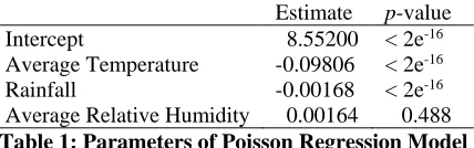
The expected dengue incidence was modeled using Poisson regression. The explanatory variables were monthly average temperature, monthly cumulative rainfall and monthly average relative humidity. The results are given in Table 1.

Estimate p-value Intercept 8.55200 < 2e-16 Average Temperature -0.09806 < 2e-16 Rainfall -0.00168 < 2e-16 Average Relative Humidity 0.00164 0.488

Table 1: Parameters of Poisson Regression Model

Before we interpret the relationship between dengue incidences and the three given climate variables, we check the goodness of fit of the model and the overdispersion. The dispersion parameter estimated to be 92.26 indicates high levels of overdispersion. This violates the assumption that the mean equals the variance in the Poisson model. The p-value of the Pearson chi-square test using deviances is 0. This proves that there is of lack of model fit.

The quasi-Poisson model was fitted on data to deal with the overdispersion of data. This model can be used for overdispersed count data and it gives the same model estimates as in the Poisson model, but standard errors are adjusted for overdispersion. Table 2 gives the parameter estimates and corresponding p-values.

Estimate p-value Intercept 8.55200 0.0048 Average Temperature -0.09806 0.1782 Rainfall -0.00168 0.0014 Average Relative Humidity 0.00164 0.9413

Table 2: Parameters of Quasi-Poisson Regression Model

Based on this model, rainfall is the only climate variable that produces a significant relation to dengue incidences. To investigate this further and to address the overdispersion of data,

∑ − − =





























2 y_{i i}

ISSN 2250-3153

we fitted the negative binomial model on data. The results are given in Table 3. The negative binomial model is a better model to fit the expected dengue incidences because the dispersion parameter given in Poisson model has been reduced from 92.26 to 1.09. The p-value of the Pearson chi-square test using deviances is 0.255 indicating adequacy of the model fit. This model also confirms that rainfall is the only significant factor influencing dengue incidences.

Estimate p-value

Intercept 8.54536 0.0004 Average Temperature -0.10858 0.1225 Rainfall -0.00179 0.0000 Average Relative Humidity 0.00566 0.7942

Table 3: Parameters of Negative Binomial Model

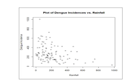
We plotted dengue incidences against the rainfall to identify any apparent association. The plot is given in Figure 1. The plot shows a weak negative association. The Pearson correlation coefficient is -0.35804 also suggesting a weak negative association.

Figure 1: Plot of Dengue Incidences against Rainfall

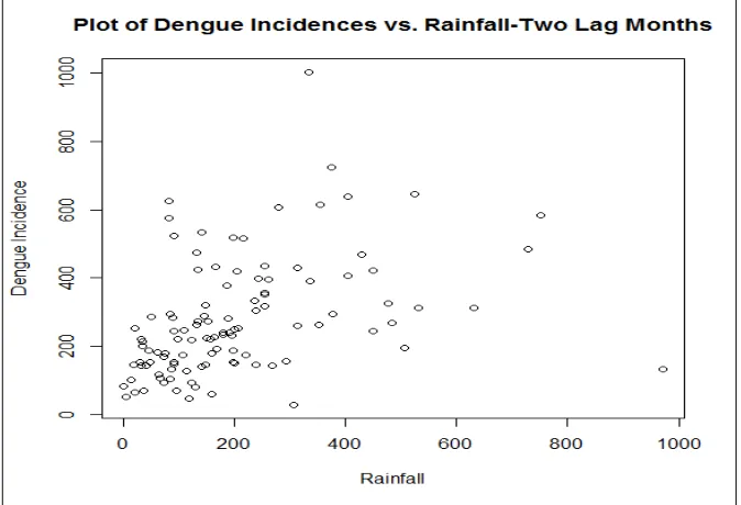
Since it takes a certain period of time for an egg to develop into an adult mosquito, the influence of climate is expected to be visible one or two months later [18]. For this reason we model monthly dengue incidences using one and two lag month’s climate data. For one lag month data, the Pearson correlation coefficient between dengue incidences and rainfall was

ISSN 2250-3153

Figure 2: Plot of Dengue Incidences against Two Lag Months Rainfall

Here onwards we considered the two lag month data for our data analysis. Then we fitted Poisson and negative binomial regression models for dengue incidences based on the three climate factors that we considered earlier. Both models indicated that the only significant factor affecting dengue incidences was the rainfall. Therefore, we dropped the non-significant climate factors, the average temperature and the average relative humidity from the model. Then we fitted models for the relationship between the dengue incidences and the rainfall. Table 4 and Table 5 give the parameter estimates of the Poisson model and the Negative Binomial model respectively:

Estimate p-value Intercept 5.360 < 2e-16 Rainfall 0.001191 < 2e-16

Table 4: Parameters of Poisson Model

Estimate p-value Intercept 5.264 < 2e-16 Rainfall 0.0016151 1.84e-07

Table 5: Parameters of Negative Binomial Model

The p-values show significant positive association in both models. The Pearson chi-square test using deviances in Poisson

model and Negative Binomial model were 0 and 0.2970 respectively. The estimated dispersion parameters for the Poisson and Negative Binomial models were 83.51 and 1.07. These values indicate that the negative binomial model is a better fit and it overcomes the overdispersion of data. The negative binomial model assumes that the conditional mean is not equal to the condition variance. Since the Poisson model is nested in the Negative Binomial model, we can also use the likelihood ratio test to compare the two models and test this model assumption. The value of the chi-square test statistic was 8274.925 (p = 0.00). This strongly suggests the negative binomial model is more appropriate than the Poisson model.

ISSN 2250-3153

Figure 3: Quantile Residuals against Fitted Dengue Incidences for Poisson Model

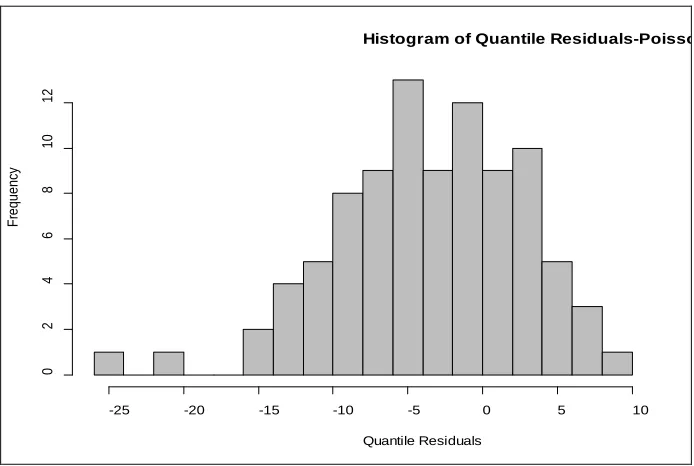
Figure 4: Histogram of Quantile Residuals for Poisson Model

200 300 400 500 600

-2

5

-2

0

-1

5

-1

0

-5

0

5

Quantile Residual Plot-Poisso

Fitted Dengue Incidences

Q

uant

ile R

es

idual

s

Histogram of Quantile Residuals-Poisso

Quantile Residuals

F

requenc

y

-25 -20 -15 -10 -5 0 5 10

0

2

4

6

8

10

ISSN 2250-3153

Figure 5: Normal Q-Q Plot of Quantile Residuals for Poisson Model

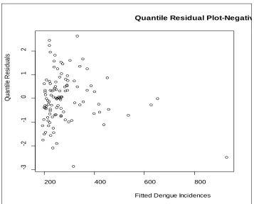
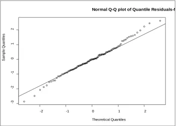
The Figures 6, 7 and 8 give the quantile residual plot, histogram, and the normal probability plot for the negative binomial model. From the residual plot and the histogram, we noticed residuals are in the range of –3 to 3. The histogram and the normal probability plot suggest residuals are approximately normally

distributed (symmetric with fat tails). Based on what we concluded using hypothesis tests earlier and the residual analysis, we determine that the negative binomial model is better for modeling dengue incidences.

Figure 6: Quantile Residuals against Fitted Dengue Incidences for Negative Binomial Model

-2 -1 0 1 2

-2

5

-2

0

-1

5

-1

0

-5

0

5

10

Normal Q-Q plot of Quantile Re

Theoretical Quantiles

S

am

pl

e Q

uant

iles

200 400 600 800

-3

-2

-1

0

1

2

Quantile Residual Plot-Negativ

Fitted Dengue Incidences

Q

uant

ile R

es

idual

ISSN 2250-3153

Figure 7: Histogram of Quantile Residuals for Negative Binomial Model

Figure 8: Normal Q-Q Plot of Quantile Residuals for Negative Binomial Model

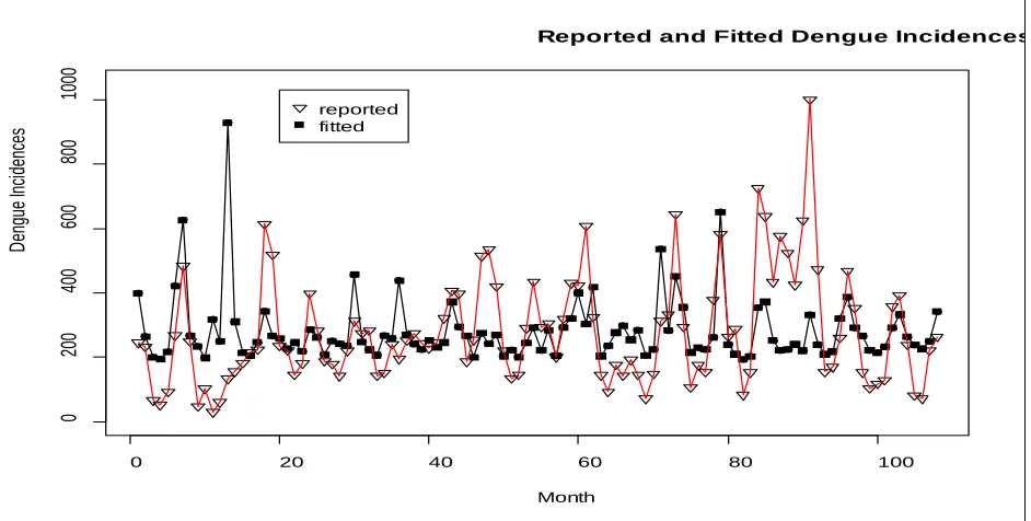
In Figure 9, we plotted the reported and fitted monthly dengue incidences using the negative binomial model from 2010 to 2018 in a same graph. This plot shows the relationship between

actual and fitted dengue incidences in Colombo, Sri Lanka during that period.

Histogram of Quantile Residuals-Negati

Quantile Residuals

F

requenc

y

-3 -2 -1 0 1 2 3

0

5

10

15

20

25

-2 -1 0 1 2

-3

-2

-1

0

1

2

Normal Q-Q plot of Quantile Residuals-N

Theoretical Quantiles

S

am

pl

e Q

uant

il

ISSN 2250-3153

Figure 9: Reported and Fitted Dengue Incidences from 2010 - 2018

Interpretation of Coefficients

We observed that the rainfall was the only significant climate variable affecting the monthly dengue incidences based on the models we considered. Furthermore, we noticed that the negative binomial regression model with two lag months rainfall data was the best model to fit the dengue incidences. Now we use this model to interpret the model coefficients. Table 5 shows the regression coefficients and p–values for this particular model. We observed that the rainfall is very significant (p-value is nearly 0) with the regression coefficient equaling to 0.0016151. For every one unit (mm) increase in amount of monthly rainfall amount, the expected dengue incidences increases by exp(0.0016151) = 1.001616 times. For every one unit increase in amount of monthly rainfall amount, the 95% confidence interval for the expected dengue incidence increment will be between 1.000929 and 1.002337 times. In other words, for each one unit rise in rainfall, the average monthly dengue incidences increases by 0.162% or for every 10 units rise in rainfall, the average number of dengue incidences increase by 1.62%.

The form of the model equation for negative binomial regression is the same as that for the Poisson regression. The log of the outcome is predicted with a linear combination of the predictors. For our model, the regression equation is given as

ln(λ) = 5.264 + 0.0016151*R

where λ is the expected dengue incidences and R stands for the amount of monthly rainfall.

Discussion

The climate of Sri Lanka, which is a part of South Asia, is mainly dominated by rainy seasons on a yearly basis. In this study we found that the rainfall significantly affects the dengue incidences. Furthermore, we observed that two lag months climate data influences the dengue incidences. Since it takes several weeks for an egg to develop into an adult mosquito, influence in climate is expected to be visible one or two months later. Once adult mosquitos have emerged, the climate factors determine their chances of survival. The increase in mosquito population due to the rainfall and subsequent increase in dengue incidences has been reported before [19].

Initially, we considered Poisson and negative binomial regression models to investigate the association between monthly dengue incidences and three climate variables, namely, average temperature, rainfall, and average relative humidity. It was revealed that the only significant variable related to the monthly dengue incidences was rainfall. Due to the overdispersion of data, the Poisson model did not fit well. The negative binomial model which is the proper model for overdispersed data was a better fit. The Pearson correlation coefficient and the scatterplot between the current month’s rainfall and the dengue incidences showed a weak negative association. The Pearson correlation coefficient and the scatterplot between dengue incidences and two lag months

0 20 40 60 80 100

0

200

400

600

800

1000

Reported and Fitted Dengue Incidences

Month

D

engue I

nc

idenc

es

ISSN 2250-3153

rainfall showed significant positive association. Since there was no apparent association between dengue incidences and the other two climate factors, average temperature and relative humidity, we drop them from our models. Then we fit the Poisson and negative binomial models to analyze the relationship between dengue incidences and two lag months rainfall. While both models showed positive association between dengue incidences and rainfall, the negative binomial model was the better fit based on dispersion parameter, likelihood ratio test and the analysis of quantile residuals. The quantile residuals are approximately normally distributed in the negative binomial model indicating a better fit.

This study showed a significant positive effect between the rainfall and the dengue incidences. Several previous studies conducted in other parts of the world also indicate similar findings [20]. The positive effect from rainfall is justifiable because rain water forms water pools which provide breeding grounds for mosquitoes. That increases the mosquito density which in turn leads to an increase in dengue incidences rates among the public. The dengue incidences may also be associated with socio-economic levels of people and the dengue control measurements implemented by the relevant authorities. These factors were not considered in our model.

V. CONCLUSION

Dengue is a critical public health problem in Colombo as well as other parts of Sri Lanka. The objective of this study was to identify the climate factors affecting the dengue incidences in the city of Colombo. The study used the monthly data from 2010 to 2018 in Colombo. The Poisson and negative binomial regression models were used to fit the data. The Poisson model did not fit the data well due to the overdispersion in the data. The negative binomial model was found to be the better fit. The results suggested that the rainfall was the only significant factor affecting dengue incidences. The negative binomial model can be used to predict the expected monthly dengue incidences based on rainfall amounts. Furthermore, we noted that the influence of rainfall on dengue incidences is expected to be visible after some lag period. These findings would be helpful to local authorities to take necessary steps to safeguard the community from dengue outbreaks.

REFERENCES

[1] CDC: Centers for disease control and prevention. https://www.cdc.gov/dengue/index.html

[2] P.P.N.N. Sirisena and F. Noordeen, “ Evolution of Dengue in Sri Lanka— Changes in the Virus, Vector, and Climate”, International Journal of Infectious diseases, Vol 19, 2014, pp. 6-12.

[3] G. N. Malavige, N. Fernando and G. Ogg, “ Pathogenesis of Dengue Viral Infections”, Sri Lankan Journal of Infection Diseases, Vol 1(1), 2011, pp. 2-8.

[4] Epidemiology Unit of Ministry of Health of Sri Lanka. http://www.epid.gov.lk/web/

[5] K. Goto, B. Kumarrendran, S. Mettananda, D. Gunasekara, Y.Fujii and S. Kaneko, “ Analysis of Effects of Meteorological Factors on Dengue Incidence in Sri Lanka Using Time Series Data”, PLOS ONE 8(5), 2013, https://doi.org/10.1371/journal.pone.0063717

[6] G. P. Withanage, S. D. Wishwakula, Y. I. Gunawardena and M. D. Hapugoda, “A Forecasting Model for Dengue Incidence in the District of Gampaha, Sri Lanka”, Parasit Vectors, 2018 Vol 11,

doi: 10.1186/s13071-018-2828-2.0

[7] H. W. B. Kavinga, D. D. M. Jayasundara and D. K. N. Jayakody , “ A New Dengue Outbreak Statistical Model using the Time Series Analysis”,

European International Journal of Science and Technology, 2(10), 2013,

pp. 35-52.

[8] W. Sun, L. Xue and X. Xie, “ Spatial-temporal Distribution of Dengue and Climate Characteristics for Two Clusters in Sri Lanka from 2012 to 2016”, Scientific Reports, Vol 7: 2017, 12884.

[9] Md. N. Karim, S. U. Munshi, N. Anwar. and Md. S.Alam, “ Climate Factors Influencing Dengue Cases in Dhaka City: A Model for Dengue Prediction”, Indian Journal of Medical Research, V136(1), 2012, pp. 32-39.

[10] Y. Hii, H. Zhu, N. Ng, L.C. Ng and J. Rocklov, “ Forecast of Dengue Incidence Using Temperature and Rainfall”, Plos Negl Trop Dis, Vol 6(11), 2012, e1908. doi: 10.1371/journal.pndt.0001908.

[11] J. A. Iguchi, X. T. Seposo. and Y. Honda, “ Meteorological Factors Affecting Dengue Incidence in Davao, Philippines”, BMC Public Health, Vol 18:629, 2018, https://doi.org/10.1186/s12889-018-5532-4.

[12] T. K. Yamana and E. A. Eltahir “ Incorporating the Effects of Humidity in a Mechanistic Model of Anopheles Gambiae Mosquito Population Dynamics in the Sahel Region of Africa”, Parasit Vectors, Vol 9(6):235, 2013, doi: 10.1186/1756-3305-6-235.

[13] Department of Census and Statistics of Sri Lanka. http://www.jjay.cuny.edu/user/login

[14] F. Moksony and R. Hegedus, “The Use of Poisson Regression in the Sociological Study of Suicide”, Corvinus Journal of Social Policy,Vol 5(2), 2014, pp.94-114.

[15] A. Zeileis, C. Klieber and S. Jackman, “ Regression Models for Count Data in R”, Journal of Statistical Software, Vol 27(8), 2008, pp.1-25. [16 ] A. Abdulhafedh, “ Crash Frequency Analysis”, Journal of Transportation

Technologies, Vol(6), 2016, pp. 169-180.

http://dx.doi.org/10.4236/jtts.2016.64017

[17] K. P. Dunn and G. K. Smyth, “ Randomized quantile residuals”, Journal of

Computational and Graphical Statistics, Vol 5,1996, pp.1-10.

http://www.statsci.org/smyth/pubs/residual.html

[18] K. Nakhapakorn and N. K. Tripathi,” An Information Value Based Analysis of Physical and Climatic Factors Affecting Dengue Fever and Dengue Haemorrhagic Fever Incidence”, International Journal of Health

Geographics, Vol 4(13), 2005, doi: 10.1186/1476-072X-4-13

ISSN 2250-3153

[20] Y. Choi, C. S. Tang, L. McIver, M. Hashizume, V. Chan, R.R. Abeyasinghe, S. Iddings and R.Huy,” Effects of Weather Factors on Dengue Fever Incidence and Implications for Interventions in

Cambodia”, BMC public health, Vol 16(241), 2016, doi:10.1186/s12889-016-2923-2

AUTHORS

First Author – Leslie Chandrakantha, Department of

Mathematics and Computer Science, John Jay College of City University of New York, New York, USA,