Image Interpolation with New Modified Eight Adjacent Regression for
High Resolution Graphics
Prashant Kushwaha
1Amit Chouksey
21
M. Tech. Scholar
2Associate Professor
1,2
Gyan Ganag College of Technology, Jabalpur, MP, India
Abstract— With bitmap graphics, as the size of an image is enlarged, the pixels that form the image become increasingly visible, making the image appear "soft" if pixels are averaged, or jagged if not. Image interpolation methods however, often suffer from high computational costs and unnatural texture interpolation. Image interpolation, which is based on an autoregressive model, has achieved significant improvements compared with the traditional algorithm with respect to image reconstruction, including a better peak signal-to-noise ratio (PSNR) and improved subjective visual quality of the reconstructed image. However, the time-consuming computation involved has become a bottleneck in those autoregressive algorithms. The main purpose of this work is to provide recursive algorithms for the computation of the Newton interpolation polynomial of a given two-variable function.
Key words: Newton Bivariate Interpolation Terms—Image Interpolation, Autoregressive Model, Parallel Optimization
I. INTRODUCTION
Image interpolation becomes pre-processing step in order to other image processing tasks like image registrations, image rotation. Image registration needs interpolation to accurately register image at sub-pixel level. Interpolation techniques are mainly divided in two categories:
Non-adaptive techniques Adaptive techniques
Non-adaptive interpolation techniques are based on direct manipulation on pixels instead for considering any statistical feature or content for an image. These are kernel based interpolation techniques where unknown pixel values are found by convolving with kernel. Hence they follow same pattern for calculation in order to all pixels. Moreover most for them are easy to perform and have less calculation cost. Various non-adaptive techniques are nearest neighbor, bilinear, bicubic, etc.
Adaptive techniques consider image feature like intensity value, edge information, texture, etc. Non-adaptive interpolation techniques have problems for blurring edges or artifacts around edges and only store low frequency components for original image. in order to better visual quality, image must have to preserve high frequency components and this job can be possible with adaptive interpolation techniques. Various adaptive techniques exists in order to image interpolation NEDI, DDT, ICBI, etc.
The interpolation is a method for enhancing image resolution means enhancing pixel data, here need to guess
new value between available pixels problem is that guessing what should be value for new pixel which will be produce a smooth and sharp highly resolute image. available procedure for image interpolation are good enough however only problem is that this methods are using linear interpolation means pixels that they develops between two pixels is computed as per mean value between two continuous pixels.
II. METHODOLOGY
Conventional bilinear interpolation (2 pixels), cubic convolution interpolation (4 pixels), cubic spline interpolation (4 adjacent pixels), these classical algorithms can lead to interpolation artifacts such as blurring, ringing, jaggies, and zippering.
To preserve edge structures in interpolation, Li and Orchard proposed to estimate the covariance of HR images from the covariance of LR images, and to then interpolate the missing pixels based on the estimated covariance.
Zhang and Wu present SAI (soft-decision adaptive interpolation) which use 2-D autoregressive model, But the core of autoregressive models was a time-cost approach, which makes it difficult to meet the requirements of real-time reconstruction in actual production.
SAI image modal can be presented as
𝑋(𝑖, 𝑗) = ∑(𝑚.𝑛)∈𝑊𝛼(𝑚, 𝑛)𝑋(𝑖 + 𝑚, 𝑗 + 𝑛)+ 𝑣𝑖,𝑗 (1)
𝛼(𝑚, 𝑛) is the autoregressive coefficient Li and Orchard SAI modal use gauss siedel regression modal to compute 𝛼(𝑚, 𝑛) Jiaji Wu et al [1] use following method to compute nine unknown pixels y1 to y9 form, sixteen know pixels using following auto-regression modal:-
A is a 16x4 matrix for the sub image as shown in below figure developed for diagonal four 8-connected neighbours.
B is 16x4 matrix for the sub image as shown in below developed for vertical four of 4-connected neighbours.
𝑎 = (𝐴𝑇𝐴)−1𝐴𝑇𝑥)
𝑏 = (𝐵𝑇𝐵)−1𝐵𝑇𝑥)
To compute 9 unknown pixels of y=[y1,y2….y9]
𝑦 = (𝐶𝑇𝐶)−1𝐶𝑇𝐷𝑥 Where
𝐶 = [𝐼9 𝐻]
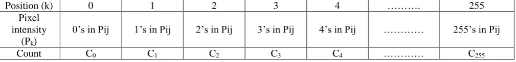
Let a non-interpolated image is 𝑃𝑖𝑗 having size of NxM, where i=1,2,3,4………….N and j=1,2,3,4…………M Histogram equalization
Position (k) 0 1 2 3 4 ………. 255
Pixel intensity
(Pk)
0’s in Pij 1’s in Pij 2’s in Pij 3’s in Pij 4’s in Pij ………… 255’s in Pij
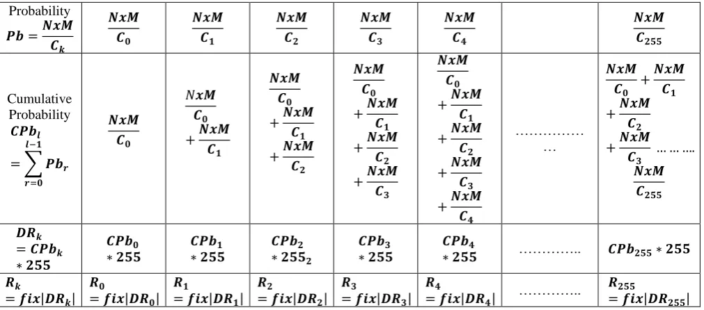
[image:1.595.47.552.692.753.2]Probability
𝑷𝒃 =𝑵𝒙𝑴
𝑪𝒌 𝑵𝒙𝑴 𝑪𝟎 𝑵𝒙𝑴 𝑪𝟏 𝑵𝒙𝑴 𝑪𝟐 𝑵𝒙𝑴 𝑪𝟑 𝑵𝒙𝑴 𝑪𝟒 𝑵𝒙𝑴 𝑪𝟐𝟓𝟓 Cumulative Probability 𝑪𝑷𝒃𝒍
= ∑ 𝑷𝒃𝒓
𝒍−𝟏 𝒓=𝟎 𝑵𝒙𝑴 𝑪𝟎 𝑁𝒙𝑴 𝑪𝟎 +𝑵𝒙𝑴 𝑪𝟏 𝑵𝒙𝑴 𝑪𝟎 +𝑵𝒙𝑴 𝑪𝟏 +𝑵𝒙𝑴 𝑪𝟐 𝑵𝒙𝑴 𝑪𝟎 +𝑵𝒙𝑴 𝑪𝟏 +𝑵𝒙𝑴 𝑪𝟐 +𝑵𝒙𝑴 𝑪𝟑 𝑵𝒙𝑴 𝑪𝟎 +𝑵𝒙𝑴 𝑪𝟏 +𝑵𝒙𝑴 𝑪𝟐 +𝑵𝒙𝑴 𝑪𝟑 +𝑵𝒙𝑴 𝑪𝟒 ……… … 𝑵𝒙𝑴 𝑪𝟎 +𝑵𝒙𝑴 𝑪𝟏 +𝑵𝒙𝑴 𝑪𝟐 +𝑵𝒙𝑴 𝑪𝟑 … … …. 𝑵𝒙𝑴 𝑪𝟐𝟓𝟓 𝑫𝑹𝒌
= 𝑪𝑷𝒃𝒌
∗ 𝟐𝟓𝟓 𝑪𝑷𝒃𝟎 ∗ 𝟐𝟓𝟓 𝑪𝑷𝒃𝟏 ∗ 𝟐𝟓𝟓 𝑪𝑷𝒃𝟐
∗ 𝟐𝟓𝟓𝟐
𝑪𝑷𝒃𝟑
∗ 𝟐𝟓𝟓
𝑪𝑷𝒃𝟒
∗ 𝟐𝟓𝟓 ………….. 𝑪𝑷𝒃𝟐𝟓𝟓∗ 𝟐𝟓𝟓
𝑹𝒌
= 𝒇𝒊𝒙|𝑫𝑹𝒌|
𝑹𝟎
= 𝒇𝒊𝒙|𝑫𝑹𝟎|
𝑹𝟏
= 𝒇𝒊𝒙|𝑫𝑹𝟏|
𝑹𝟐
= 𝒇𝒊𝒙|𝑫𝑹𝟐|
𝑹𝟑
= 𝒇𝒊𝒙|𝑫𝑹𝟑|
𝑹𝟒
= 𝒇𝒊𝒙|𝑫𝑹𝟒|
………….. 𝑹𝟐𝟓𝟓
= 𝒇𝒊𝒙|𝑫𝑹𝟐𝟓𝟓|
Rij is Histogram Equalized image can be obtain form Pij by
𝑲′𝒔 𝒑𝒊𝒙𝒆𝒍 𝒊𝒏𝒕𝒆𝒏𝒔𝒊𝒕𝒚 𝒐𝒇 𝑷
𝒌= 𝑹𝒌 𝒘𝒉𝒆𝒓𝒆 𝒌 =
𝟎, 𝟏, 𝟐, … … 𝟐𝟓𝟓
HSV stretching 𝑻𝒊𝒋= 𝑹𝑮𝑩𝟐𝑯𝑺𝑽(𝑹𝒊𝒋)
let R,G and B are the pixels of red, green and blue frames of Rij
H=
{
𝑼𝒏𝒅𝒆𝒇𝒊𝒏𝒆 𝒊𝒇 𝑴𝑨𝑿 = 𝑴𝒊𝒏
𝟔𝟎𝑿 𝑮−𝑩
𝑴𝑨𝑿−𝑴𝑰𝑵+ 𝟎 𝒊𝒇 𝑴𝑨𝑿 = 𝑹 𝒂𝒏𝒅 𝑮 ≥ 𝑩
𝟔𝟎𝑿 𝑮−𝑩
𝑴𝑨𝑿−𝑴𝑰𝑵+ 𝟑𝟔𝟎 𝒊𝒇 𝑴𝑨𝑿 = 𝑹 𝒂𝒏𝒅 𝑮 < 𝑩
6𝟎𝑿 𝑩−𝑹
𝑴𝑨𝑿−𝑴𝑰𝑵+ 𝟏𝟐𝟎 𝒊𝒇 𝑴𝑨𝑿 = 𝑮
𝟔𝟎𝑿 𝑹−𝑮
𝑴𝑨𝑿−𝑴𝑰𝑵+ 𝟐𝟒𝟎 𝒊𝒇 𝑴𝑨𝑿 = 𝑩
S={𝟎 𝒊𝒇 𝑴𝑨𝑿 = 𝟎 𝟏 −𝑴𝑰𝑵
[image:2.595.47.553.66.289.2]𝑴𝑨𝑿 𝒐𝒕𝒉𝒆𝒓𝒘𝒊𝒔𝒆 V=MAX
Fig. 1: Image interpolation neighbours
{𝑿𝒊𝒋}𝟔𝒙𝟔= {𝑻𝒊𝒋} 𝒇𝒐𝒓 𝒊 = (𝒆: 𝒆 + 𝟓) , 𝒋
= (𝒇: 𝒇 + 𝟓) 𝒘𝒉𝒆𝒓𝒆 𝒆 = 𝟏: 𝟔: 𝑵 𝒂𝒏𝒅 𝒇 = 𝟏: 𝟔: 𝑴
A is a 16x4 matrix isolated from the sub image of
𝑿𝒊𝒋 for diagonal four 8-connected neighbours.
B is 16x4 matrix isolated for the sub image for vertical four of 4-connected neighbours.
𝒂 = (𝑨𝑻𝑨)−𝟏𝑨𝑻𝒙)
𝒃 = (𝑩𝑻𝑩)−𝟏𝑩𝑻𝒙)
To compute 9 unknown pixels of y=[y1,y2….y9]
𝒚 = (𝑪𝑻𝑪)−𝟏𝑪𝑻𝑫𝒙 Where
𝐱 = [𝐱𝟏, 𝐱𝟐 … . 𝐱𝟏𝟔]𝑻
𝑪 = [𝑰𝟗 𝑯]
And
H =
a1 a2 0 a3 a4 0 0 0 0 0 a1 a2 0 a3 a4 0 0 0 0 0 0 a1 a2 0 a3 a4 0 0 0 0 0 a1 a2 0 a3 a4 0
-b1𝝀 0
-b3𝝀 1
-b4𝝀 0
-b2𝝀 0
And
𝝀 = ∑ {[
∑𝟑𝒊=𝟏𝒂𝒊
𝟖 +
∑𝟑𝒊=𝟏𝒃𝒊 𝟖 ] − 𝒂𝒊
𝟒 ⁄ }
𝟑
𝒊=𝟎 And
By putting value of D, H, 𝝀 , C and x the values of unknown pixels y can be computed from equation above and obtain full sub image will be of 11x11 the same process will continue for the next sub-image of 6x6 and generate a new sub image of 11x11
C
1 0 0 0 0 0 0 0 0
0 1 0 0 0 0 0 0 0
0 0 1 0 0 0 0 0 0
0 0 0 1 0 0 0 0 0
0 0 0 0 1 0 0 0 0
0 0 0 0 0 1 0 0 0
0 0 0 0 0 0 1 0 0
0 0 0 0 0 0 0 1 0
0 0 0 0 0 0 0 0 1
0 0 0 0 a1 a2 0 a3 a4 0 -b1𝝀 0 -b3𝝀 1 -b4𝝀 0 -b2𝝀 0
D a 1
a
2 0 0 a 3
a
4 0 0 0 0 0 0 0 0 0 a
1 a
2 0 0 a 3
a
4 0 0 0 0 0 0 0 0 0 a
1 a
2 0 0 a 3
a
4 0 0 0 0 0 0 0 0 0 a
1 a
2 0 0 a 3
a
4 0 0 0 0 0 0 0 0 0 a
1 a
2 0 0 a 3
a
4 0 0 0 0 0 0 0 0 0 a
1 a
2 0 0 a 3
a
4 0 0 0 0 0 0 0 0 0 a
1 a
2 0 0 a 3
a
4 0 0 0 0 0 0 0 0 0 a
1 a
2 0 0 a 3
a 4 0 0 0 0 0 0 0 0 0 a
1 a
2 0 0 a 3
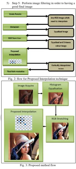
a 4 0 0 0 0 0 1 0 0 0 0 0 0 0 0 0 0 0 0 0 0 1 0 0 0 0 0 0 0 0 0 0 0 0 0 0 0 0 1 0 0 0 0 0 0 0 0 0 0 0 0 0 0 1 0 0 0 0 0 0 0 0 0 0 0 0 0 0 0 0 0 Figure 2 below shows flow for proposed interpolation technique it is been seen that available methods for interpolation does not concerns about original image quality if original image is not good than its interpolated image will also be not good. So proposed work is concerning about it and first enhancing original image quality than performing interpolation, Proposed block diagram is shown above, flow for proposed algorithm as follow:-
1) Step 1: capture or choose any image in any YUY or RGB format, image should be a low resolution image which we require to interpolation.
2) Step 2: perform histogram equalization in order to equalized distribution for colour quality; histogram equalization is a popular procedure in order to performing equalised
3) Step 3: perform HSV (Hue, Saturation amd Value) stretching is in order to enhancing quality for image, MAX is maximal value in R, G, B for all pixels in image, and MIN is minimal one.
H=
{
𝑼𝒏𝒅𝒆𝒇𝒊𝒏𝒆 𝒊𝒇 𝑴𝑨𝑿 = 𝑴𝒊𝒏
𝟔𝟎𝑿 𝑮−𝑩
𝑴𝑨𝑿−𝑴𝑰𝑵+ 𝟎 𝒊𝒇 𝑴𝑨𝑿 = 𝑹 𝒂𝒏𝒅 𝑮 ≥ 𝑩
𝟔𝟎𝑿 𝑮−𝑩
𝑴𝑨𝑿−𝑴𝑰𝑵+ 𝟑𝟔𝟎 𝒊𝒇 𝑴𝑨𝑿 = 𝑹 𝒂𝒏𝒅 𝑮 < 𝑩
𝟔𝟎𝑿 𝑩−𝑹
𝑴𝑨𝑿−𝑴𝑰𝑵+ 𝟏𝟐𝟎 𝒊𝒇 𝑴𝑨𝑿 = 𝑮
𝟔𝟎𝑿 𝑹−𝑮
𝑴𝑨𝑿−𝑴𝑰𝑵+ 𝟐𝟒𝟎 𝒊𝒇 𝑴𝑨𝑿 = 𝑩
S={𝟎 𝒊𝒇 𝑴𝑨𝑿 = 𝟎 𝟏 −𝑴𝑰𝑵
𝑴𝑨𝑿 𝒐𝒕𝒉𝒆𝒓𝒘𝒊𝒔𝒆 V=MAX
4) Step 4: Perform Proposed interpolation as explain above it will produce a horizontally interpolated image.
[image:3.595.303.554.63.620.2]5) Step 5: Perform image filtering in order to having a good final image
Fig. 2: flow for Proposed Interpolation technique
Fig. 3: Proposed method flow
III. RESULTS
Mean Squared Error (MSE) Definition: mean squared error MSE for an estimator is one from many types to quantify & difference between values used by an estimator & actual values for quantity being estimated. MSE measures averages for squares for errors.MSE should be less in order to better performance.
let D is data, C is cipher, len is length for data, MSE: Mean Square Error , SNR: Signal to Noise ratio
[image:3.595.46.281.63.463.2]Peak Signal-to-noise ratio (PSNR) Definition: PSNR is a measurement that compares level for a required signal to level for background noise. It is defined as ratio for actual signal power to noise power, often expressed in decibels. SR should be high in order to better performance for design system
𝑷𝑺𝑵𝑹 = 𝟐𝟎𝒍𝒐𝒈𝟏𝟎𝑴𝑺𝑬̅̅̅̅̅̅̅ 𝟐𝟓𝟔𝟐
propose work has done simulation for the target MATLAB standard images of Lena, Barbara, Cameraman and peppers, this images taken for the test of proposed work because the exact same images were taken by the base works [1] to [10].
Image name Before Interpolation After interpolation Size Pixels Size Pixels Lena 8 Kb 225x225 372 Kb 2022x2022 Barbara 100 Kb 512x512 1.92
Mb
4605x4605
Peppers 12 Kb 225x225 348 Kb 2022x2022 Cameraman 8 Kb 204x204 260 Kb 1833x1833
Table 1: Observe results of the test images
from table 1 above it can be observe that the size of the all test images increases and also the number of pixels increases using proposed method hence interpolation has been done as was expected now it has to be observe that new develop images are having same information as it was in its original or not, for that we need to measure MSE and PSNR between original and interpolated image.
[image:4.595.343.510.147.216.2]Image name PSNR MSE Lena 38.9498 0.7395884 Barbara 41.69 0.5394 Peppers 43.8010 0.4230886 Cameraman 34.16 0.6238
Table 2: PSNR and MSE results of the test images table 2 above shows the observe PSNR and MSE for all test images it can be seen that the average PSNR is approximately 40 db which signifies that the very less amount of changes between original and interpolated.
Table 3 show the comparative results between propose work and Jiaji Wu [1], Tudor Barbu [2], Shuyuan Zhu [3], Delibasis [4], Kazu Mishiba [5] and Lei Shu[8] works for the test images of Lena, Barbara, Peppers and Cameraman, the comparison parameter is PSNR.
Image name
Proposed work PSNR
Jiaji Wu [1]
Tudor Barbu [2]
Shuyuan Zhu [3]
Delibasis [4]
Kazu Mishiba [5]
Lei Shu [8]
Lena 38.9498 32.96 34.84 31.62 35.46 35.1025
Barbara 41.69 22.22 25.66
Peppers 43.8010 31.27
Cameraman 34.16 26.14 27.50
Table 3: PSNR comparison for test images from the table 3 and figure 7 it can be clearly observe
that the proposed work PSNR is better than available work for all test images, it is because of proposed new interpolation method which is been discussed earlier.
IV. CONCLUSION
As interpolation is technique which is used in order to improving and modification for image, video or any other data, so many interpolation techniques are been developed in area, basically interpolation was application for signal processing now it has versatile uses. Proposed work is new idea for doing interpolation which includes a mathematical procedure developed in order to finding approximation here we have used that procedure in order to finding empty pixel value or pixel which is to be interpolated. procedure is using eight beside pixels to computer one unknown pixel. Proposed work is a new concept for using approximation procedure in order to image interpolation, many old and latest methods are available and all for it using various signal processing methods like nearest neighbour, linear interpolation, bicubic etc. few methods uses sinc function and various standard windows (harr, keiser, barlett etc.) however all for this methods were computing new pixel with either 1pixel or 2 pixel or 4 pixel however our procedure is computing new pixel with 8 pixels and so new pixels generated in proposed work is much accurate than other methods.
Proposed work has achieve better results than available work and we can conclude that after implementation for our defined approach for interpolation we will have very good and better quality for image as desired
order to method not higher than existing work and proposed work has achieve better SNR and MSE then existing work. Inage Interpolation can be used for enhancing image quality. Proposed work has explored limits for Interpolation practice & theory. Improvement for image interpolation system using approximation approach is providing a good quality image. A
approximation has been used to system during interpolation and in near future few other approximation procedure can be implemented. Or may possible to develop new approximation procedure proposed procedure is using one 2 dimension interpolation row wise an column wise in near future it can be in frame for image.
REFERENCES
[1] Jiaji Wu, Long Deng, Gwanggil Jeon, Image Autoregressive Interpolation Model using GPU-Parallel Optimization, IEEE TRANSACTIONS ON INDUSTRIAL INFORMATICS (ACCEPTED MANUSCRIPT: TII-17-0340), DOI 10.1109/TII.2017.2724205, IEEE-2017
[2] Tudor Barbu, Structural Image Interpolation using a Nonlinear Second-order Hyperbolic PDE-based Model,
The 6th IEEE International Conference on E-Health and Bioengineering - EHB 2017, June 22-24, 2017
[3] X. Li and M. T. Orchard, “New edge-directed interpolation,” IEEE Trans. Image Processing, vol. 10, no. 10, pp. 1521–1527, 2001.
[5] X. Wu, X. Zhang, and X. Wang, “Low bit-rate image compression via adaptive down-sampling and constrained least squares upconversion,” IEEE Trans. Image Processing, vol. 18, no. 3, pp. 552–561, 2009. [6] K. Tang, O. C. Au, Y. Guo, J. Pang, J. Li, and L. Fang,
“Arbitrary factor image interpolation by convolution kernel constrained 2-D autoregressive modeling,” in Proc. ICIP, 2013, pp. 996–1000.
[7] W. Dong, L. Zhang, R. Lukac, and G. Shi, “Sparse representation based image interpolation with nonlocal autoregressive modeling,” IEEE Trans. Image Processing, vol. 22, no. 4, pp. 1382–1394, 2013. [8] R. G. Keys, “Cubic convolution interpolation for digital
image processing,” IEEE Trans. Acoustics, Speech and Signal Processing, vol. 29, no. 6, pp. 1153–1160, 1981. [9] H. S. Hou and H. Andrews, “Cubic splines for image
interpolation and digital filtering,” IEEE Trans. Acoustics, Speech and Signal Processing, vol. 26, no. 6, pp. 508–517, 1978.
[10]L. Mussi, F. Daolio, and S. Cagnoni, “Evaluation of parallel particle swarm optimization algorithms within the CUDATM architecture,” Information Sciences, vol. 181, no. 20, pp. 4642–4657, 2011.
[11]J. Wu, Z. Song, and G. Jeon, “GPU-parallel implementation of the edge directed adaptive intra-field deinterlacing method,” Journal of Display Technology, vol. 10 no. 9, pp. 746–753, 2014.
[12]B. Huang, J. Mielikainen, H. Oh, and H.-L. A. Huang, “Development of a GPU-based high-performance radiative transfer model for the Infrared Atmospheric Sounding Interferometer (IASI),” Journal of computational Physics, vol. 230, no. 6, pp. 2207–2221, 2011.
[13]N. Zhang, Y.-s. Chen, and J.-l. Wang, “Image parallel processing based on GPU,” in Proc. ICACC, 2010, vol. 3, pp. 367–370.
[14]X. Jia, Y. Lou, R. Li, W. Y. Song, and S. B. Jiang, “GPU-based fast cone beam CT reconstruction from undersampled and noisy projection data via total variation,” Medical Physics, vol. 37, no. 4, pp. 1757– 1760, 2010.