Jaswinder Lota†, FHEA, SMIEEE; M.Al-Janabi*, MIEEE; Izzet Kale*, MIEEE †School of Architecture Computing& Engineering, University of East London
London, United Kingdom; [email protected] *
Department of Electronic, Communication & Software Engineering University of Westminster, London, United Kingdom [email protected], [email protected]
Abstract-The present approaches on predicting stability of Delta-Sigma (Δ-Σ) modulators are mostly confined to DC
inputs. This poses limitations as practical applications of Δ-Σ modulators involve a wide range of signals other than DC. In this paper, a quasi-linear model for Δ-Σ modulators with nonlinear feedback control analysis is presented that accurately predicts the stability of higher-order single-loop 1-bit Δ-Σ modulators for various types of input signals such as single-sinusoids, dual-sinusoids, multiple-sinusoids and Gaussian. Theoretical values are shown to match closely with simulation results. The results of this paper would significantly speed up the design and evaluation of higher-order single-loop 1-bit Δ-Σ modulators for various applications including those that may require multiple-sinusoidal inputs or any general input composed of a finite number of sinusoidal components, circumventing the need to perform detailed time-consuming simulations to quantify stability limits. By using the proposed method, the difference between the predicted and the actual stable amplitude limits results in an error of less than 1 dB in the in-band Signal-to-Noise Ratio (SNR) for 3rd- and higher-order Δ-Σ modulators for single-sinusoidal inputs. For single-, dual-, multiple-sinusoidal and Gaussian inputs the error is less than 2 dB for the 5th-order and reduces to less than 1 dB for 6th- and higher-order Δ-Σ modulators.
Index Terms—delta-sigma, stability analysis, non-linear systems, multiple inputs
I. INTRODUCTION
The stable input amplitude limits for Delta-Sigma (Δ-Σ) modulators are complicated to predict due to the non-linearity of the quantizer. The stable input amplitude limit decreases as the order of the Δ-Σ modulator increases. One technique is to model the quantizer as a threshold function in the state equations, which gets complicated for higher-order Δ-Σ modulators and is limited to 1st- and 2nd- order Δ-Σ modulators [1]. Another approach to simplify the analysis has been to assume a DC input to the Δ-Σ
Nonlinear model based approach for accurate
stability prediction of one-bit higher-order
2
error of less than 1 dB in the in-band Signal-to-Noise Ratio (SNR) for 3rd- and higher-order Δ-Σ modulators for single-sinusoidal inputs. For single-, dual-, multiple-sinusoidal and Gaussian inputs the error is less than 2 dB for the 5th-order and reduces to less than 1 dB for 6th- and higher-order Δ-Σ modulators.
The results from this novel model would significantly speed up the design and evaluation of higher-order Δ-Σ modulators for numerous applications including those that may require multiple-sinusoidal inputs or any general input composed of a finite set of sinusoidal components. The method would facilitate a detailed testing of a given Δ-Σ modulator based Analog-to-Digital Converter (ADC) or a Digital-to-Analog Converter (DAC) with arbitrary test signals generated from a combination of multiple-sinusoids without having to go through the actual excitation of the Δ-Σ modulator with real and lengthy raw signals. As an example, speech signals that may be generated from the combination of five sinusoids, using this method would circumvent the need to feed real speech signals into the ADC and undertake lengthy simulations to establish the stability limits. The only requirement here would be to feed the model developed with the set of five sinusoid combinations to have very rapid results. Section II describes the stability mechanism in terms of the quasi-linear model and the Noise Amplification Factor. Section III elaborates on the concept of the ratio of the signal variance to the quantization noise variance at the quantizer input followed by the variation of quantization noise in the Δ-Σ modulator. Subsequently a comparative analysis for the multiple- and the single-sinusoidal inputs is undertaken. Simulations are given in Section IV, followed by conclusions in Section V.
II. QUASI-LINEAR Δ-Σ MODULATOR AND NOISE AMPLIFICATION FACTOR
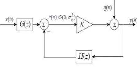
[image:3.612.196.419.539.649.2]A quasi-linear model of a Δ-Σ modulator is shown in Fig.1, where G(z) is the input transfer function, H(z) the feedback filter transfer function and the quantizer is replaced by a gain factor K followed by an additive white quantization noise source q(n):
Fig. 1. Quasi-linear Δ-Σ modulator.
Assuming q (n) to be white with a zero mean and variance σq2, and the Noise Transfer Function (NTF) between q(n) and y(n) to
4
[image:4.612.182.429.224.415.2](1) where, A(K) is the Noise Amplification Factor. Using Parseval’s theorem, A(K) can also be found in the time-domain as in [12]:
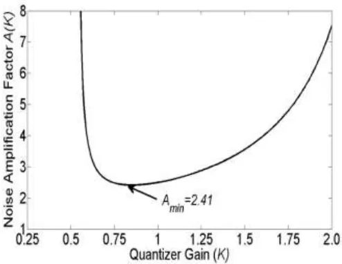
(2) where ntf(n)is the impulse response corresponding to NTF(z) and ||ntf||22 is the squared second-norm of ntf(n). The variation of A(K) with K can be plotted as A(K) curves from (2) and is used to explain the stability of Δ-Σ modulators. A typical curve for a 4th-order Δ-Σ modulator is shown in Fig. 2, where Amin is the global minimum value of the curve which is 2.41.
Fig. 2. Noise Amplification Factor variation with quantizer gain.
The Δ-Σ modulator is considered to be stable in the positive slope section of the A(K) curve. If K increases slightly in this section of the curve, which is monotonically increasing, then A(K) will increase. This results in higher noise amplification leading to more noise circulating in the Δ-Σ modulator loop. Higher quantization noise power tends to decrease K, which in turn decreases A(K) and the system is therefore in equilibrium. In the negative slope section of the curve however, such an equilibrium does not exist and even small perturbations would destabilize the system. Therefore, for stable operation, the Δ-Σ modulator must operate in the positive section of the slope. It would be seen as per the analysis undertaken that as the input amplitude increases, A(K) continues to decrease, until A(K) reaches Amin. At this point the Δ-Σ modulator commences operation in the negative section of
the slope and hence becomes unstable. For stable operation of the Δ-Σ modulator therefore, A(K) > Amin.[12]. If one can quantify the variation of A(K) with the input signal amplitude a for which A(K)> Amin, then the maximum stable input amplitude limits
can be established. Quantifying A(K) is done in two steps, first by estimating the ratio of signal variance to quantization noise variance at the input to the quantizer gain K and subsequently by estimating the variation of quantization noise variance σq2 with
III. SIGNAL AND NOISE VARIANCE AT QUANTIZER INPUT AND QUANTIZATION NOISE
A. The ratio of the signal variance to quantization noise variance at the quantizer input.
Consider a signal with a Gaussian PDF at the quantizer input with variance σex2. If σeq2 is the variance of the quantization noise at
the input to the quantizer and the signal and quantization noise are uncorrelated then the combined variance at the quantizer input is given by:
(3)
The quantizer gain K of a Δ-Σ modulator for a Gaussian input with variance σe2 for a single-bit output is given by [18]:
(4)
Defining ρ2 as the ratio of the signal variance to the quantization noise variance at the quantizer input, yields the equation below: (5)
The quantizer gain K can be found from (3), (4) and (5) as given by:
(6)
From Figure 1 we have:
As the Signal Transfer Function (STF) of the Δ-Σ modulator should ideally be ≈ 1, therefore . From (7) we have:
From (8) it follows that:
(9) As ∆ can be assumed to be equal to 1 for a single-bit quantizer, one gets the following relationship from (5), (6) and (9):
(10)
For a single-sinusoidal input with amplitude a, the signal variance is given by . From (10) one can obtain an equivalent relationship:
(11)
Consider an input signal consisting of N multiple incommensurate sinusoids with the variances σi
2
, i=1,2,…N. For example,
6
number of sinusoids as the input signal variance can be incremented accordingly. The input signal variance for the dual-sinusoidal input is given by:
(12) For the dual-sinusoidal input from (10) and (12), one obtains:
(13) For a multiple-sinusoidal input with N = 5, the input signal variance is given by:
(14) For the multiple-sinusoidal input from (10) and (14), one can obtain:
(15)
Equivalently from (10) for a Gaussian signal with an input variance one gets:
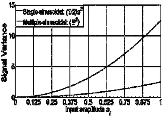
(16) By solving (11), (13), (15) and (16), one can get ρ for the various types of input signals which are plotted in Fig. 3. The signal amplitude a for the dual/multiple-sinusoidal input corresponds to the sum of the amplitudes of the sinusoids and for the Gaussian input, it corresponds to the standard deviation of the input signal. It is observed that ρ increases almost linearly for the single-sinusoidal input but nonlinearly for the multiple-single-sinusoidal and Gaussian inputs for a > 0.6 as shown in Fig. 3.
Fig. 3. Variation of and .
B. Quantization noise variance.
If E(.) is the expectation operator, the power at the output of the Δ-Σ modulator is given by:
(18) Assuming ∆ as ±1 for the single-bit quantizer, the quantization noise variance σq2 is obtained from (18) and is plotted for various
types of inputs as shown in Fig. 3. The quantization noise variance is found to be the same in all cases. This is expected, as the quantization noise power in the ∆-Σ loop should depend on the number of quantizer bits, which is unity in this case. Assuming
the quantization noise to be uniformly distributed between ±∆ implies a variance of [2]. This is 0.33 for a quantizer, whose ∆ values are ±1. The amplitude of the quantization noise variance from Fig. 3 is 0.36.
C. Noise Amplification Factor.
Thenoise variance at the output of a Δ-Σ modulator is:
(19) From (6) and (19), one gets:
(20) The variation of A(K) with a can be found by (1) and (20), which is given as:
(21)
Using (21),A(K) is plotted in Fig. 4 for various input signals. It decreases as a increases reaching Amin at which point the Δ-Σ
modulator becomes unstable. From (1) is directly proportional to the NTF, which is dependent on the Δ-Σ modulator order, the higher the order, the bigger becomes. From (1) and (21), it is seen that as the Δ-Σ modulator order increases, so does Vo
thereby increasing Aminin Fig. 2. Thus, the Δ-Σ modulator becomes unstable at lower amplitudes for higher NTF orders. On the
other hand, as the number of quantizer bits increases, the quantization noise variance σq
2
8
Fig. 4. Variation of A(K ) with signal input amplitude/standard deviation.
The values obtained for the single-sinusoid are higher than those for the multiple-sinusoidal inputs. This is because the signal variance at the input to the quantizer is higher for a single-sinusoid with an amplitude a than for a multiple-sinusoid with equal amplitudes. This is illustrated by the variation of with for i=5 in Fig.5.
Fig. 5. Variation of and .
[image:8.612.160.448.420.638.2]input to the quantizer would be much lower for five sinusoids with equal amplitudes of 0.14 than for a single-sinusoidal input with an amplitude of 0.7, the 3rd-order Δ-Σ modulator is likely to be stable for a > 0.7 for the multiple-sinusoidal input. This is observed from the A(K) values for the single-sinusoidal input shown in Fig. 4, which are obtained from (20), wherein the A(K) values for the single-sinusoidal input are lower than the multiple-sinusoidal A(K) values. This results in the Δ-Σ modulator reaching the unstable limits at lower values of a for the single-sinusoidal input.
IV. SIMULATION RESULTS
A. Simulation Results.
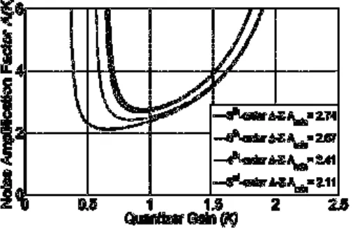
[image:9.612.182.435.309.474.2]Simulations were undertaken for 3rd-, 4th-, 5th- and 6th-order single-loop single-bit Δ-Σ modulators. The corresponding A(K) curves for these Δ-Σ modulators are shown in Fig 6. The Amin values for the curves are 2.11, 2.41, 2.67 and 2.74 respectively.
Fig.6. Variation of Noise Amplification Factor with quantizer gain.
[image:9.612.170.443.577.714.2]The Δ-Σ modulators were implemented by deploying a cascade-of-accumulators feedback-form (CAFB) topology as shown in Fig. 7 for the 4th-order Δ-Σ modulator case.
10
The coefficient values for the Δ-Σ modulators are shown in Table I. The coefficients were obtained using the Matlab based delta-sigma toolbox in [22].
TABLEI
COEFFICIENTS FOR Δ-ΣMODULATORS
Δ Σ i 1 2 3 4 5 6 7
6th-order
δi 0.0003 0.0055 0.0423 0.2001 0.6104 1.1151 1.0000
αi 0.0003 0.0055 0.0423 0.2001 0.6104 1.1151 -
βi 1.0000 1.0000 1.0000 1.0000 1.0000 1.0000 -
γi 0.0001 0.0011 0.0021 - - - -
5th-order
δi 0.0028 0.0334 0.1852 0.5904 1.1120 1.0000 -
αi 0.0028 0.0334 0.1852 0.5904 1.1120 - -
βi 1.0000 1.0000 1.0000 1.0000 1.0000 - -
γi 0.0007 0.002 - - - - -
4th-order
δi 0.0157 0.1359 0.5140 0.3609 1.0000 - -
αi 0.0157 0.1359 0.5140 0.3609 - - -
βi 1.0000 1.0000 1.0000 1.0000 - - -
γi 0.003 0.0018 - - - - -
3rd-order
δi 0.0751 0.0421 0.9811 1.0000 - - -
αi 0.0751 0.0421 0.9811 - - - -
βi 1.0000 1.0000 1.0000 - - - -
γi 0.0014 - - - -
The multiple-sinusoidal input signal consists of five incommensurate sinusoid amplitudes, which are increased in steps of 0.0003. The sinusoids are selected at random frequencies of 1 kHz, 3.25 kHz, 5.5 kHz, 7.5 kHz and 8 kHz. For comparison with the single-sinusoidal input, the frequency chosen is 8 kHz and for the dual-sinusoidal input, the frequencies are 5.5 kHz and 8 kHz to ensure the same Over-Sampling Ratio (OSR). The simulation parameters for the Δ-Σ modulators are an OSR of 32 and a sampling frequency of 512 kHz. All the initial conditions of the Δ-Σ modulators are set to zero. In order to have the number of FFT input samples as a power of 2, a simulation time of 4.096 seconds is used giving 2097152 FFT samples at the Δ-Σ modulator output. The SNR is obtained by plotting the FFT Power Spectral Density (PSD) using a Hanning window. The SNR increases as a increases and the SNR for the single-sinusoidal input remains higher than the multiple- sinusoidal input due to the greater signal variance. As the variance of the signal at the quantizer input is also higher, the 3rd-order Δ-Σ modulator becomes unstable at a lower value of a= 0.66thanit does for the multiple-sinusoidal input for a = 0.99. At a = 0.66, it starts to fall showing the onset of instability for the single-sinusoidal input. The numerical stable value of a as predicted from Fig. 4 is 0.68, when A(K) = 2.11 = Amin. The predicted stable value of 0.68 is very close to the 0.66 obtained via simulations. The SNR for the
seconds on an Intel® Core™ 2 Duo 2.26 GHz processor, operating with Windows 7 2009 and Matlab version 7.7.0.471(R2008b). This is for varying K from 0.01 to 2.8 in steps of 0.01 giving a total of 280 plot points. For a single 4.096 second simulation, the time required is 35 seconds. As the amplitude is varied in smaller steps of 0.0003 for rigorous quantification, a total of 1100 simulations are required to reach the stable amplitude limit of 0.33 for the multiple-sinusoidal input for the 5th-order Δ-Σ modulator resulting in a net simulation time of 4505 seconds. Therefore the simulation time is reduced from 4505 seconds to 7 seconds, which is a reduction of over 99 %. Higher stable limits are expected for the 3rd- and 4th-order Δ-Σ modulator leading to even further increases in the simulation time, while there is marginal change in the simulation time for the A (K) curves for the Δ-Σ modulators.
B. Accuracy of Results.
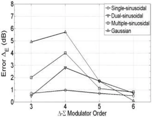
The numerically predicted stable limits along with the ones obtained via simulations are shown in Table II. For the single-sinusoidal, dual-sinusoidal and multiple-sinusoidal inputs, the error ∆Ein dB represents the in-band SNR error due to the
difference between the numerically predicted input signal amplitudes and those obtained via simulations. For the Gaussian input, it indicates the error in the predicted variance and that obtained via simulations at the Δ-Σ modulator input for the stable limits of operation.
TABLEII
SIMULATION VALUES
Single-sinusoidal Order Stable Limit Error ∆E
(dB) Simulated Numerically
Predicted
III 0.66 0.68 0.71
IV 0.47 0.49 0.96
V 0.21 0.23 0.7
VI 0.07 0.075 0.5
Dual-sinusoidal III 0.7 0.95 0.5
IV 0.45 0.70 2.8
V 0.24 0.34 1.7
VI 0.07 0.08 0.72
Multiple-sinusoidal III 0.99 1.55 2.00
IV 0.61 1.30 4.00
V 0.33 0.38 1.10
VI 0.15 0.19 0.8
Gaussian Variance
Simulated Numerically Predicted
III 0.07 0.22 4.9
IV 0.032 0.12 5.7
V 0.0054 0.0081 1.7
VI 0.000175 0.00018 0.1
The variation of the error (∆E) versus the ∆-Σ modulator order is plotted in Fig. 8. It is observed that ∆E is less than 1 dB for 3rd-,
12
modulator order increases from 3 to 4, the rate of increase in SNR with the signal amplitude increases, thereby resulting in a higher increase in the values of ∆E. Although the rate of increase in the SNR continues as the order is further increased from 4 to
6, ∆E reduces to less than 1 dB because the characteristics of the quantization noise become more Gaussian-like as the modulator
[image:12.612.179.424.151.340.2]order is increased. This result validates (4) and the subsequent analysis.
Fig. 8 Error (∆E) variation with ∆-Σ modulator order.
V. CONCLUSIONS
REFERENCES
[1] Hein, S., and Zakhor, A.: ‘On the stability of sigma-delta modulators’, IEEE Trans. on Signal Processing, Jul 1993, Vol. 41, No.7, pp. 2322-2348.
[2] Ardalan, S. H., and Paulos, J.J.: ‘An analysis of non-linear behaviour in Σ-Δ modulators’, IEEE Trans. on Circuits and Systems, Jun 1987, Vol. CAS-34, No. 6, pp. 1157-1162.
[3] Steiner, P., and Yang, W.: ‘Stability analysis of the second-order sigma-delta modulator’. Proc. IEEE Int. Sym. on Circuits and Systems-ISCAS 94, 1994, Vol. 5, pp. 365-368.
[4] Fraser, N. A., and Nowrouzian, B.: ‘A novel technique to estimate the statistical properties of sigma-delta A/D converters for the investigation of DC stability’. Proc. IEEE Int. Symp. on Circuits and Systems-ISCAS 02, May 2002, Vol.3, pp.111-289-111-292.
[5] Wong, N., and Tung-Sang, N.G.: ‘DC stability analysis of higher-order, lowpass sigma-delta modulators with distinct unit circle NTF zeroes’, IEEE Trans. on Circuits & Systems-II: Analog and DSP, Vol. 50, Issue 1, Jan 2003, pp. 12-30.
[6] Zhang, J., Brennan, P.V., Juang, D., Vinogradova, E., and Smith, P.D.: ‘Stable boundaries of a 2nd-order sigma-delta modulator’. Proc. South. Symp.
on Mixed Signal Design, Feb 2003, pp. Feb 2003.
[7] Zhang, J., Brennan, P.V., Juang, D., Vinogradova, E., and Smith, P.D.: ‘Stable analysis of a sigma-delta modulator’. Proc. IEEE Int. Symp. on Circuits and Systems-ISCAS 03, May 2003, Vol.1, pp.1-961-1-964.
[8] Reefman, D., Reiss, J. D., Janssen, E., and Sandler, M. B.: ‘Description of limit cycles in sigma-delta modulators’, IEEE Transactions on Circuits and Systems I, June 2005, Volume 52, Issue 6, p.1211 – 1223.
[9] Reiss, J.D: ‘Towards a procedure for stability analysis of higher-order sigma-delta modulators’. 119th Audio Engineering Society (AES) Convention, Oct 2005, New York, USA.
[10]Angus., J. A. S.: ‘A comparison of the ‘pruned-tree’ versus ‘stack’ algorithms for look-ahead sigma–delta modulators,’ Journal of the Audio Engineering Society, vol. 54, pp. 477-494, 2006.
[11]Reiss, J.D.: ‘Understanding sigma delta modulation: the solved and unsolved issues,’ Journal of the Audio Engineering Society, vol. 56, pp. 49-64, 2008.
[12]Risbo, L.: ‘Stability predictions of higher-order delta-sigma modulators based on quasi-linear modeling’. Proc. IEEE Int. Symp. on Circuits and Systems-ISCAS 94, 30 May-02 Jun 1994, Vol.5, pp. 361-364.
[13] Lota, J., Al-Janabi, M., and Kale, I.: ‘Stability analyses of higher-order delta-sigma modulators using the Describing Function method’. Proc. IEEE Int. Symp. on Circuits and Systems-ISCAS 2006, May 2006, pp. 593-596.
[14] Lota, J., Al-Janabi, M., and Kale, I.: ‘Stability analyses of higher-order delta-sigma modulators for dual-sinusoidal inputs’. Proc. IEEE Inst. and Measurements Technology Conf.-IMTC 2007, Warsaw, Poland, pp. 1-5.
[15] Lota, J., Al-Janabi, M., and Kale, I.: ‘Nonlinear stability analyses of higher-order sigma-delta modulators for DC and sinusoidal inputs’, IEEE Trans. on Inst. and Measurements, Mar 2008, Vol. 57, No. 3, pp. 530-542.
[16] Altinok, D.G., Al-Janabi, M., and Kale, I.: ‘Stability analysis of bandpass sigma-delta modulators for single- and dual-tone sinusoidal input’, IEEE Trans. on Inst. and Measurements, Feb 2011, Vol. 60, Issue 5, pp. 1546-1554..
[17] Lota, J., Al-Janabi, M., and Kale, I., ‘Accurate stability prediction of single-bit higher-order Δ-Σmodulators for Speech Codecs,’ Proc. IEEE
International Symposium on Circuits & Systems -ISCAS 2011, Rio de Janeiro, Brazil, 15-18May 2011.
[image:13.612.67.573.50.711.2][18] Gelb, A., and Velde, W. E. V.: ‘Multiple-Input Describing Functions and Nonlinear System Design’ (McGraw-Hill Book Company), Appendix E Table of Random-Input Describing Functions (RIDFs), pp. 565-588, 1968.
[19] Foote, K.G., and D.T.I, Francis.: ‘Scheme for parametric sonar calibration by standard target’. Proc. IEEE/MTS OCEANS 2005, Vol. 2, pp. 1409-1414, Sept 2005.
[20] Foote, K.G., Patel, R., and Tenningen, E.: ‘Target-tracking in a parametric sonar beam, with applications to calibration’. Proc. IEEE/MTS OCEANS 2010, pp. 1–7, Dec 2010.
[21] Bjorno, L.: ‘Developments in sonar and array technologies’. 2011 Proc. IEEE Symp. on Underwater Technology (UT), and 2011 Workshop on Scientific Use of Submarine Cables and Related Technologies (SSC), pp. 1 – 11, Apr 2011.