An Adaptive Scheduling System for Computational Grid
using Autonomic Computing
Ebrahim Aghaei
Department of Computer
Engineering, Science and
research Branch,
Islamic Azad University
Khouzestan-Iran
Mohammad Saniee
Abadeh
Electrical and Computer
Engineering Faculty,
Tarbiat Modares University
Tehran
Mohammad Hossein
Yektaie
Department of IT,
Faculty of Technology and
Engineering, Qom University
Gom
ABSTRACT
Grid computing provides an environment to be share software and hardware resources.Ontheonehand, environmentofGridcomputingis inherently large, complex, heterogeneous and dynamic and its state changes over time, on the other hand, incoming job to Grid show unstable behavior, which before that is not known and changes over time. As regards that scheduling in Grid has a vital role in overall system performance, the need to scheduling methods to adapt themselves to conditions in Grid, and regarding current state of the environment and jobs the scheduler must be able to make decisions. In this article, for the scheduling of computational Grid, we have used Autonomic Computing principles to enable Grid scheduler dynamically adapt itself totheenvironmentandincreaseefficiency. Autonomic computing systems are inspired by biologically systems which their goal is to manage themselves with minimal involvement of managers. Autonomic computing is suitable for a computational Grid because of the large, heterogeneous, dynamic and autonomous nature of the Grid. The proposed method in this study, in terms of makes pan, execution time and resource utilization has shown higher performance, compared to other methods and related numerous experiments.
General Terms
Adaptive Algorithms, Grid Scheduling, Autonomic Grid.
Keywords
Computational Grid, Grid Scheduling, Adaptive Scheduling, Autonomic Computing.
1.
INTRODUCTION
TheGridisanemerginginfrastructurethatusefromnumerousresou rcesacrosstheworldassharedmanner[1]. Anyone from anywhere in the world can easily be connected to the Grid and uses a numerous computing resources and communicationresourcessharedittorunhis(her)applications.
Using of different types of computing resources via computer networks and the Internet, allow us able to much use of their capabilities. Using these infrastructures, we have the capability that can be shared distributed resources across the world to solve very large problems in many different fields of science and industry. The research was done in this area, has emerged the paradigm of distributed computing which today is known as Grid.
Grid execution environments and applications have characteristics that have distinguished them from other traditional infrastructure [2][3]. Some of these characteristics of Grid are: Heterogeneity in Grid, which shows Grid environments composed of large numbers of different independent computational resources which geographically distributed in the world (supercomputers, personal computers, services and so on), and Similarly, applications typically combine multiple independent components or services which Each have their own specific requirements. The next characteristic of Grid is Dynamism. The Grid environment is continuously changing; at any moment of time may a resource add to system or failure; Applications similarly have dynamic runtime behaviors and they can change in any time. Complexity is other characteristic of Grid. Whatever system is larger and composed of various components, have more complexity. The Grid can be expanded in the whole world; So, Such a system has much complexity which it may be difficult to management. Today, a fundamental problem facing managers is the complexity of the Grids. Uncertainty is other characteristic of Grid. Uncertainty in Grid environment is caused by multiple factors, including dynamism, failures, and incomplete knowledge of global system state [2]. Uncertainty in Grid causes which cannot consider static states for the Grid. Finally, Security is a critical challenge in these environments, because on the one hand, an application could have security requirements and, on the other hand, the Grid resource could have their own security requirements.
Due to these characteristics, management of Grid based on passive components and static states is not practical. Clearly, the need to consider many of fundamental issues, to its management and configure be easier. These issues have caused researchers to turn to principles of management techniques, which are able to dynamically adapt themselves to existing conditions. The resulting approach is called autonomic computing, which its purpose is to provide the computing systems which are able to manage themselves with minimal human intervention managers [4][5]. By changing in the environment of autonomic systems (i.e. human body), the system makes action to fit it and take away it to another correct state. An autonomic system or application offers features awareness, definition, healing, self-configuring, self-optimizing and self-protection and so on. This is known as self-* features [6].
Grid, and the scheduler should be aware of these changes as soon as possible to make the best decision. In the Grid may be resources added to the system or leave it at any time. In addition, various errors may occur in any moment of time. These errors can be resources errors, network errors, application errors and so on. Therefore, the use of static algorithms in such system would be problematic. We need to dynamic algorithms for scheduling which could use of the latest information, and adapt themselves with suchenvironment.Mostexistingschedulingalgorithms,notconsi der to conditions and changes has been in Grid which this causes the scheduler to make the wrong decisions.
In this paper we have presented an architecture based on the principles of autonomic computing for computational Grid scheduling. Using the proposed method, the scheduler can as soon as be aware of changes and errors generated in the Grid and based on information obtained make better decisions. In each period, scheduler uses the best available resources and does not use inefficient resources. Our proposed method takes into consideration this fact which sometimes may be a resource with high performance become a resource with low performance (based on existing conditions), and vice versa, some of the resources with low performance become resources with higher performance. This means that our proposed method do not consider a constant state for resources and assume that resources are changing over time.
The remainder of this article is structured as follows. Section 2 describes the issues that are about the scheduling in Grid. Section 3 shows the principle of autonomic computing and Section 4 describes the proposal that was formulated to solve an issue we identified during investigation. Section 5 reveals an evaluation of the proposal, and finally Section 6 mentions some of the conclusions that can be drawn from all of this work.
2.
GRID SCHEDULING
The scheduling of jobs to heterogeneous resources in Grid is a well-known NP-hard problem, and various sub-optimal solutions have been proposed [7][8][9][10][11]. When a single job arrives at a Grid within a unit scheduling time slot, the scheduling system will analyze the load situation of every resources and select one resource to run this job.
The process of allocation a resource to a job involves three basic phases and each phase involves several steps [12]. In the first phase, the resources currently available in the Grid are identified and all the required information of the resources must be collected and store in a database. The Scheduler, use of available resource information to determine the resource is able to run which jobs. This information can include: resource operating system, resources speed, bandwidth between the scheduler and the resource, cache memory size of the resource, the current load of the resource, the current availability of the resource and so on.
In the second phase, a resource from the available resources is chosen by using a scheduling algorithm and the job assign to that. All resources could not be candidates for the allocation of jobs. Therefore, the selection process is carried out based on job requirements and resource characteristics. The scheduling algorithm tries to maximize some optimization criterion specified by the user or by the system. This criterion can be throughput, response time,
The third phase of Grid scheduling is running a job. In this phase, the job is migrated to the selected resources and executed on it. This phase is called job migration[13].
Depending on the job and its running time, users may monitor the progress of their job and possibly change their mind about where or how it is executing. Historically, such monitoring is typically done by repetitively querying the resource for status information, but this is changing over time to allow easier access to the data. If a job is not making sufficient progress, it may be rescheduled or migrated to other resources.
3.
AUTONOMIC COMPUTING
Autonomic Computing is a term coined by IBM, and its goal is realizing computing systems and applications capable of managing themselves with minimum human intervention [4] [5][14].Autonomic computing is inspired by the human autonomic nervous system that handles complexity and uncertainties. The human nervous system is an evolved great example of natural autonomous behavior. This system is able to balance the body and keep it in steady state. Autonomic systems represent an appropriate response to any change in the environment to that always system remains in a stable balanced state.
3.1
Autonomic Computing Architecture
IBM has to offer reference architecture for autonomic computingwhich is composed of several basic components[14]. These components work together to that adapt themselves to current conditions. These components are composition together to that provides a service in accordance with the policies of the application or system, and continuously and dynamically they can adapt themselves to changes over time. The next section provides a brief description of the autonomic computing to the concept is obvious[15][16][17][18].
IBM described several components (layer) for autonomic system. These components include manual managers, autonomic managers, touchpoints and managed resources that they use a share knowledge source. Manual manager is an interface for the IT professional through it specifies high level policies of system; this component will produce an overall plan and uses it to guide application and system and determines forthem how to act to achieve an optimal healthy state.
Function of autonomic manager is production and execution a plan based on predefined policies and existing conditions. Autonomic manager do work in lower level then manual manager and often is considered as the core an autonomic system. This component monitors information of the system andmanageit based on occurred change. The internal structure of an autonomic manager includes four functions: monitor, analyze, plan and execute with knowledge. These functions compose a loop called MAPE-K. The monitor function collects the information from the managed resources, via sensors. The analyze function use the information obtained from monitor function and analyze them to determine whether need to change or not. In plan function a desired plan selected or created. Finally, the desired plan execute, via effectors. This loop repeated to system adapts itself with existing conditions.
A touchpoint is an interface which links the autonomic manager to the managed resource. This link can be through sensors or effectors. Sensors enable autonomic manager to observesystem's behavior, and effectors, let autonomic manager modify the behavior of system.
server, storage unit, database, service, application or other entity.
Variouscomponents can obtain and share knowledge via knowledge sources. The various components can receive necessary information from the knowledge sources and update that, if necessary.
4.
SCHEDULING SYSTEM
ARCHITECTURE
Our proposed system has a User Interface module (UI), Global Scheduler module (GS) and Grid Information System
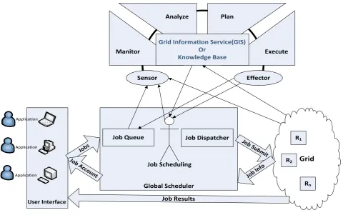
(GIS), which on above them placed the layer ofself-management which uses the principles of autonomic computing. All system components, share the information through Grid Information System (in principle of autonomic computing know knowledge base). The components of the proposed scheduling system are shown in Fig 1.
Grid
R1
R2
Rn
User Interface
Global Scheduler Job Queue
Jobs
Job Accoun
t
Job Sub
mit
Job I nfo Job Scheduling
Job Dispatcher
Job Results
Manitor
Analyze Plan
Execute Grid Information Service(GIS)
Or Knowledge Base
Sensor Effector
Application
Application
[image:3.595.58.539.196.497.2]Application
Fig 1: Proposal algorithm architecture
The UI module provides an environment which users are able to deliver their applications and then taking over required results. Through this interface, users can obtain informationabout how to run the assignedapplications.Also, to inform user, using it for progress report, occurred errors, account and etc. With running applications, results obtained are delivered to the user. The UI module, after receiving the user's applications, converts into one or more jobs, and then delivers job(s) to the GS.
GIS module collects information about the status of resources, the status of jobs, status job queue and etc. Resources informationcan be architecture, operating system, speed, workload, number of processors, amount of memory, communication bandwidth and etc. The information in this module must become updated periodically. Updated information in this module has a vital role in the Grid scheduling;because if does not reach updated Information to the scheduler, last changes are not considered and the schedulerwill make wrong decisions. Thus, available informationin this component in the decision-making scheduleris very effective.
GS moduleis divided into three sub modules the Job Queue, the Job Scheduler and the Job Dispatcher. After that UI
moduledelivered jobs to GS, they are entering to Job Queue. Job Queue sub module is used for storing ready jobs. This queue, keeps lists of jobs that are currently not able to run in Grid (may be currently have not sufficient resources). Jobs queuing can be done based on different levels of jobs priority.
Job Scheduling submoduleisresponsibleforallocatingavailabler esourcestoreadyjobs. JobSchedulerreceives latest informationof system from the GIS and makes decision accordingto jobs in the job queue. The Job Scheduler tries to selectmost appropriate resource(s) to execute the jobs, to increase the utilization of resources and jobs be executed with high speed.
The Job Dispatching sub module dispatches the job to the resource that will execute it. This sub module receives the job from the Job Scheduler module and sends it to the corresponding resource(s) to run in the resource(s).
4.1
Proposed System Structure
work in dynamic environment and many uncertainties of Grid. The structure of proposed system is shown in Fig 1. In this section, we first describes how collect information in proposed method and then describes how to schedule.
4.1.1
Collect Information in Proposed Method
We in proposed architecture used of a hybrid push-pull method for collecting information; means, informationreceives from resource and placed in theGIS(pull), and resources themselves send some of information forGIS(push).
On the one hand, self-managinglayer,atregularperiods,collects information from the Grid and store in GIS. Monitor function is responsible for collecting information. Monitor function obtained this information through the sensors. The collected information is given to analyze function, to if needed appropriate plan is executed. In the large systems of Grid,for that communication bandwidth, too much does not spend information transfer; Sources can be divided into several domains. In each domain, end Resources send informationto the intermediate resource in that domain, and self-managing layer at the end of period receives resources informationfrom this intermediate resource. In this case, does not need to get all resources information; self-managing layer can only get information changeable such as current load resources,the amount of available memory and etc., to the communication bandwidth wasted in vain.
When a resource has left the system without previous notice or a resource has failure, self-managing layer can detect it very quickly and stores in GIS; because in each period, informationobtains from Grid.
Self-managing layer could change period in a dynamic mode; means period could become low and high over time. The reason for this is that if the changes source's dynamic information is a lot, then information should store faster in GIS, to Scheduler be able use them. If the changes is low, resources information are collected at longer period, to communication bandwidth wasted in vain.
On the other hand, resources themselves have a duty which some of information send to the GIS. This mode can be used for the following: A resource add to Grid, the resource with the prior notice leaves the Grid, the resource Want to report specific information or an error, and some of the non-dynamic properties of resources are subject to change.
4.1.2
The Proposed Scheduling
Our proposed scheduling is Scheduling using the principles of Autonomic Computing (SAC). In the proposed method, the UI module, receive user's applications and divides them into one or more jobs and adds this jobs to the job queue sub module. Then job scheduling sub module receives jobs information from job queue sub module. Jobs information can be jobs number, jobs type, jobs length, type of requirements resource and etc. also, this sub module receives resources informationfrom GIS. After that necessary information received from the GIS and the job queue, scheduler decide based on requirements of entered jobs and based on current status of resources and assign jobs to appropriate resources.
Scheduler in each period receives the necessary information from the GIS and based on equation 1 calculates current amount of resources capability:
𝑳𝑺
𝒓 𝒕,𝒕 + 𝒑 = 𝑺
𝒓∗ 𝟏 − 𝑳
𝒓 𝒕,𝒕 + 𝒑 𝟏
Where t is current time and p is the size of the period; Sr is the
speed of resource r, Lr(t,t+p) is current load of resource r
inperiod t to t+p. also, LSr(t,t+p( is amount of resource
capability r in period t to t+p. As you can see in the equation 1, LSr(t,t+p) is calculated based on speed and current load of
resource.
After that scheduler received updated information from the GISin each period, calculates the LS Matrix (see Fig 2). Then, the Scheduler sorts the LS matrix in descending order to be achieved SLS matrix. When SLS was obtained, the largest job in the job queue can be assigned to the first resource in the SLS. The second largest job assigned to the second resource in the SLS. Assigning of jobs to the next period will continue the same form (For that small jobs not suffer from starvation can be used a method like the aging). As explained, the Scheduler assigns each job to the available resource with largest current capability. If in a given period, to allappropriate resource one job allocated, again assignment is repeated from the first resource (in circular). If the Resource has a high workload or Resource may not be able to do this job, the next Resource in SLS will select. High limit of the resource load specify with resources owners or system administrator (e.g. 95%). If current load of resource exceeds from specified High limit, Scheduler will not assign any job to that Resource and this operation repeated until the Resource load will be return to an acceptable level.
If in a period all resources have computational overhead, Does not allocation any of resource to jobs And jobs must wait until the next period.
If in a period, any of resource is not suitable for execution of job, Next job in the job queue is chosen and execution of that job done on the next period.
t
1t
0t
2...
t
m-1t
mR
2R
1...
R
nW
2(t
0-t
1)
W
n(t
0-t
1)
W
1(t
0-t
1)
time
W
1(t
1-t
2)
W
2(t
1-t
2)
... ...
W
n(t
1-t
2)
...
...
...
...
W
1(t
m-1-t
m)
W
2(t
m-1-t
m)
W
n(t
m-1-t
m)
...
S
1S
2...
S
nS
W
t
1t
0t
2...
t
m-1t
mSW
2(t
0-t
1)
SW
n(t
0-t
1)
SW
1(t
0-t
1)
time
SW
1(t
1-t
2)
SW
2(t
1-t
2)
... ...
SW
n(t
1-t
2)
...
...
...
...
SW
1(t
m-1-t
m)
SW
2(t
m-1-t
m)
SW
n(t
m-1-t
m)
...
[image:5.595.76.515.75.241.2]SW
Fig 2: Obtain current capability of resources
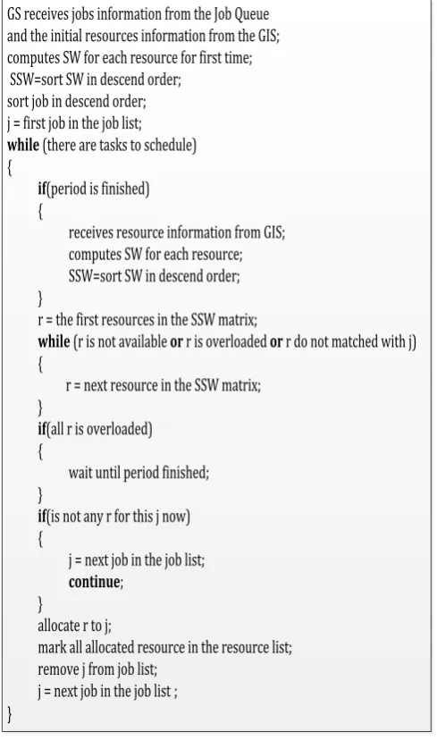
Our proposed algorithm is shown in Fig 3.
GS receives jobs information from the Job Queue
and the initial resources information from the GIS;
computes SW for each resource for first time;
SSW=sort SW in descend order;
sort job in descend order;
j = first job in the job list;
while
(there are tasks to schedule)
{
if
(period is finished)
{
receives resource information from GIS;
computes SW for each resource;
SSW=sort SW in descend order;
}
r = the first resources in the SSW matrix;
while
(r is not available
or
r is overloaded
or
r do not matched with j)
{
r = next resource in the SSW matrix;
}
if
(all r is overloaded)
{
wait until period finished;
}
if
(is not any r for this j now)
{
j = next job in the job list;
continue
;
}
allocate r to j;
mark all allocated resource in the resource list;
remove j from job list;
j
next job in the job list ;
=
}
Fig 1: Proposed algorithm
5.
A ILLUSTRATIVE EXAMPLE
Consider a Grid environment with four resources R1, R2, R3
and R4 and a job group J with eight jobs J1, J2, J3, J4, J5, J6,
J7and J8. Initially resources speed is respectively 20, 10, 15
and 5. Period is assignment three jobs to resources.
You can see assignment of jobs to resources in the period t0 to
t1 in Fig 4. After that LS matrix obtained based on S and L
and arrangement based on resources capability specify in the SLS, The biggest job in the list (J3) is assigned to the first
resource in SLS (R1). The second biggest job (J3) is assigned
to the next resource in the SLS (R3). Assignment of jobs to
resources is repeated until the period does end. If in a period, allocated job to all the resources in the SLS, assignment starts again from the first resource.
t1
t0
R2
R1
R4
20
10
5
S L(%)
Jobs Lenght
J1 J2 J3 J4 J5 J6 J7 J8
t1
LS
t0
J3
J8
J6
R3
R2
R1
R4
R3
10 8 90 3 30 43 18 89
Resource
t1
t0
(a)
(b) (c)
15 28
30
47 42
14.4
7
2.65 8.7
(1)
(2)
(3)
[image:5.595.54.299.315.729.2]SLS=(R1,R3,R2,R4)
Fig 2: Assignment of jobs to resources in the period t0 to t1
After that a period finished or a resource reported new information to the GIS, GIS information is received again and the operation is repeated. In t1 to t2 period is assumed that
speed of resource R4 has increased from 5 to 12 and current
load of resource R3 has reached to 98%. Although speed of R3
is more than R2 and R4, But in this period, does not allocated
any jobs to resource R3, because current load of this resource
[image:5.595.309.548.474.630.2]performance or worse, job failed. As you can see in Fig 5, biggest current job (J5) to first resource in SLS (R4), second
job (J7) to second resource (R2) And the third job (J1) to third
resource (R1) are assigned.
t2
t1
R2
R1
R4
20
10
12
S L(%)
Jobs Lenght
J1 J2 J4 J5 J7
t2
LS
t1
J1
J7
J5
R3
R2
R1
R4
R3
10 8 3 30 18
Resource
t2
t1
(a)
(b) (c)
15 80
37
25 98
4
6.3
9 0.3
(1) (2) (3)
SLS=(R4,R2,R1,R3)
[image:6.595.54.290.124.285.2]Changed Speed
Fig 3:Assignment of jobs to resources in the period t1 to t2
In period t2 to t3, is assumed that R2 disabled, and R1 and R3
are also very high workload. Scheduler decides that in this period jobs only assign to resource R4, because Assignment of
jobs to other resources brought down system performance. Operations in period t3 to t4 are shown in Fig 6.
t3 t2 R2
R1
R4 20
X
12
S L(%)
Jobs Lenght J2 J4
t3 LS
t2
J4 J2 R3
R2 R1
R4 R3
8 3
Resource
t3 t2
(a)
(b) (c)
15 99
X
30 96
0.2
X
8.4 0.6
(1) (2)
[image:6.595.302.550.293.505.2]SLS=(R4,R3,R1)
Fig 4:Assignment of jobs to resources in the period t2 to t3
6.
RESULTS AND DISCUSSIONS
For simulate and evaluate the proposed method, we have used the Matlab software. The environment of Grid is simulated with several independent jobs and several heterogeneous resources. We have assumed which applications users are divided into one or more independent job and add to the job queue. In different experiments, number of jobs is from 1 to 100,000. In each experiment, the jobs length generated in a specify range and randomly. The range of jobs length has been considered from 1,000 to over 1,000,000,000. The Resource speed assigned randomly in the range of is 1000000 to 1,000,000,000. Periods in the range of 0.001 to 0.01 seconds in change.
In proposed method is used current load of resources; for this reason, in each period current load of each Resource is determined randomly in range of 1 to 100. Current load each Resource is expressed in percentage. If load of a resource is set to 20, Means Currently of 20 percent capacity of Resource used and other 80 percent is not used; and if the load of resource is 100, Means that 100 percent capacity of Resource is used currently.
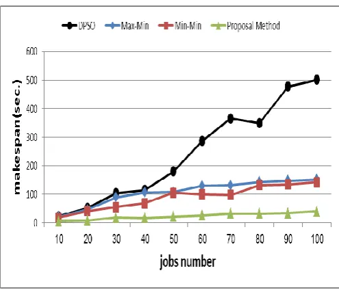
Experiments have been run on the computer with the Intel architecture, speed 2.5 GHz and 4 GB of memory. Proposed algorithm has been compared with several well-known algorithms in the field of Grid computing, such as Min-Min, Max-Min and DPSO [19] and their results are shown in Figs 7 to 9. Our evaluation is based on makespan, execution time and average resource utilization. Because of random inputs and reduce noise in results, Experiments is performed with 50 repetitions per set of input And their average is shown.
In figure7,thecomparison based on themakespanis shown. Becauseofconsiderationresourcesload, the proposed methodislessfluctuated and better results are obtained.
Fig 5: makespan
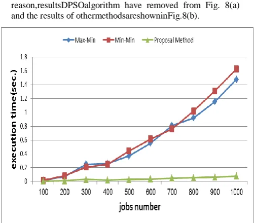
[image:6.595.56.288.403.568.2]Fig 6(a): Execution time
Because of DPSO algorithm execution time is high,in Fig.
8(a) the proposedmethod has not
beenclearlycomparedwithother methods. For this reason,resultsDPSOalgorithm have removed from Fig. 8(a) and the results of othermethodsareshowninFig.8(b).
Fig 7(b): Execution time
One another important criterion in the evaluation of Grid scheduling is resource utilization. The purpose of this criterion is that use of all available resources efficiently. This criterion can be used to demonstrate the load balancing in the system. We have calculated the average utilization of resources based on Equation 2:
𝐚𝐯𝐞𝐫𝐚𝐠𝐞
𝐮𝐭𝐥𝐢𝐳𝐚𝐭𝐢𝐨𝐧=
𝐫 𝛆 𝐫𝐞𝐬𝐨𝐮𝐫𝐜𝐞𝐜𝐨𝐦𝐩𝐥𝐞𝐭𝐢𝐨𝐧 𝐫
𝐦𝐚𝐤𝐞𝐬𝐩𝐚𝐧. 𝐫𝐞𝐬𝐨𝐮𝐫𝐜𝐞𝐍𝐮𝐦𝐛𝐞𝐫
(𝟐)
In Equation 2, completion[r] is the time of last completed job executed in each source, makespan is the largest completion
[image:7.595.41.291.69.275.2]time between resources and resourceNumber is total number of resources.
Fig 8: resource utilization
As you can see in Fig 6, our proposed method provides better average resources utilization than the other of methods.ReasonDPSOalgorithmhasworseresults than othermethods, a shorttime to decide.Becausesuch heuristicalgorithmsrequirestoo much time to better results.
7.
CONCLUSIONS
Due to the inherent complexity, heterogeneous and dynamism of Grid systems, achieving large-scale distributed computing in Grids turns out to be an elaborated work. One way for this problem is using autonomic computing, which can change its behavior in response to changes in the status of the system. We have presented an architecture which merges Grid scheduling with automatic computing techniques in order to provide self-managing behavior.
This paper presented a novel methodology for Grid scheduling using autonomic computing.We propose an autonomicGrid scheduling architecture as a possible solution, which can make scheduling decisions based on the current status of the system. Scheduler can make a decision according to the latest information obtained which can be achieved better results. We consider the load of computing resources to the best resource for execution the job is chosen in each period.
[image:7.595.315.557.97.290.2] [image:7.595.43.294.362.582.2]8.
REFERENCES
[1] I. Foster and K. Kesselman, 2004, The Grid 2: Blueprint for a New Computing Infrastructure, 2nd ed., Morgan Kaufmann Publishers.
[2] M. Parashar, H. Liu and et al., 2006, "AutoMate: Enabling Autonomic Applications on the Grid",Cluster Computing, vol. 9, no. 2, pp. 161-174.
[3] Y. Gaoa, H. Rongb and J. Z. Huangc, 2005, "Adaptive grid job scheduling with genetic algorithms",Future Generation Computer Systems, vol. 21, no. 1, pp. 151-161, October 2005.
[4] J. O. Kephart and D. M. Chess, 2003, "The Vision of Autonomic Computing",Computer, vol. 36, no. 1, pp. 41-50.
[5] S. Hariri, B. Khargharia and et al., 2006, "The Autonomic Computing Paradigm",Journal of Cluster Computing, vol. 9, no. 1, pp. 5-17.
[6] M. Rahman, R. Ranjan and R. Buyya, 2010, "A Taxonomy of Autonomic Application Management in Grids",16th IEEE International Conference on Parallel and Distributed Systems, pp. 189-196.
[7] F. Xhafa and A. Abraham, 2010, "Computational models and heuristic methods for Grid scheduling problems",Future Generation Computer Systems, vol. 26, no. 4, pp. 608-621.
[8] T. D. Braunt, H. J. Siegel and et al., 2001, "A Comparison of Eleven Static Heuristics for Mapping a Class of Independent Tasks onto Heterogeneous Distributed Computing Systems",Journal of Parallel and Distributed Computing, vol. 61, no. 6, pp. 810-837. [9] J. Yu, R. Buyya and K. Ramamohanarao, 2008,
"Workflow Scheduling Algorithms for Grid Computing",Metaheuristics for Scheduling in Distributed Computing Environments, vol. 146, pp. 173-214. [10]D. I. G. Amalarethinam and P. Muthulakshmi, 2011, "An
Overview of the Scheduling Policies and Algorithms in
Grid Computing",International Journal of Research and Reviews in Computer Science, vol. 2, no. 2, pp. 280-294. [11]H. Casanova, M. Kim and et al., 1999, "Adaptive
Scheduling for Task Farming with Grid Middleware",International Journal of High Performance Computing Applications, vol. 13, no. 3, pp. 231-240. [12]J. M. Schopf, 2003, "Ten actions when grid scheduling",
in Grid resource management Management: State of the Art and Future Trends, first ed., Springer, pp. 15-23. [13]T. Altameem and M. Amoon, 2010, "An Agent-Based
Approach for Dynamic Adjustment of Scheduled Jobs in Computational Grids",Journal of Computer and Systems Sciences International, vol. 49, no. 5, pp. 765-772. [14]IBM White Paper, 2005,"An Architectural Blueprint for
Autonomic Computing", 3th ed., IBM Corporation.
[15]M. Parashar and S. Hariri, 2007,"Autonomic Computing Concepts, Infrastructure, and Applications", CRC Press, Taylor & Francis Group.
[16]R. Nou, F. Julia and et al., 2011, "A path to achieving a self-managed Grid middleware",Future Generation Computer Systems, vol. 27, no. 1, pp. 10-19.
[17]M. Salehie and L. Tahvildari, 2009, "Self-adaptive software: Landscape and research challenges",ACM Transactions on Autonomous and Adaptive Systems, vol. 4, no. 2, pp. 1-42.
[18]M. C. Huebschr and J. A. Mccann, 2008, "A survey of Autonomic Computing — degrees, models and applications",ACM Computing Surveys, vol. 40, no. 3, pp. 1-31.