Forecasting international bandwidth capability

Forecasting international bandwidth

capability

Madden, Gary G and Coble-Neal, Grant

Curtin University of Technology, Perth, Australia

2005

Online at

https://mpra.ub.uni-muenchen.de/10822/

Forecasting International

Bandwidth Capability

GARY MADDEN* AND GRANT COBLE-NEAL

Curtin Business School, Australia

ABSTRACT

M-competition studies provide a set of stylized recommendations to enhance forecast reliability. However, no single method dominates across series, leading to consideration of the relationship between selected data characteristics and the reliability of alternative forecast methods. This study conducts an analysis of predictive accuracy in relation to Internet bandwidth loads. Extrapolation techniques that perform best in M-competitions perform relatively poorly in predicting Internet bandwidth loads. Such performance is attributed to Internet bandwidth data exhibiting considerably less structure than M-competition data. Copyright © 2005 John Wiley & Sons, Ltd.

key words bandwidth; forecast comparisons

INTRODUCTION

M-competition outcomes due to Makridakis and Hibon (1979, 2000), Makridakis et al. (1982, 1993) provide much information. These stylized outcomes, as summarized by Makridakis and Hibon (2000), are: statistically simpler models perform better than complex methods; ranking of compet-ing methods varies across accuracy measures; combincompet-ing forecasts perform best; and accuracy depends on the forecast horizon. Clements and Hendry (2001) contrast these conclusions with their theoretical research that demonstrates for weakly stationary processes, a congruent, encompassing model in-sample, based on causal variables, performs best for forecast horizons. Further, the prac-tice of pooling forecasts does not enhance accuracy.

The conflicting results of forecast performance obtained from theoretical predictions and the stylized results of M-competitions are due to the non-stationary and evolving nature of data being modelled by M-competition participants (Clements and Hendry, 2001). Simple models, they argue, offer adaptability while complicated models are susceptible to structural breaks. Moreover, these data are not reducible to stationarity through differencing. More generally, Fildes and Ord (2002) indicate that prior knowledge of the data-generating process permits a link to be established between particular data characteristics and the forecast reliability of alternative methods.

The link between the underlying properties of the data and forecast performance is explored in Fildes (1992) and Fildes et al. (1998). In examining a set of 263 telecommunications time series,

*Correspondence to: Gary Madden, Communications Economics and Electronic Markets Research Centre, School of Economics and Finance, Curtin University of Technology, GPO Box U1987, Pert, WA, Australia.

Fildes (1992) concludes that Robust Trend, developed specifically to forecast the telecommunica-tions series, performs best. Additionally, Fildes et al. (1998) provide a framework to compare and contrast the respective properties of the telecommunications and M-competition data. The use of a common set of summary statistics allows Fildes et al. to observe the relative performance of methods in relation to data characteristics. For example, they attribute an increased random component of the M-competition data to the relative decline in Robust Trend performance.

Following Fildes et al., this paper provides further information on the link between exhibited data characteristics and forecast reliability of methods. In doing so, a direct comparison with the earlier results is permitted. Moreover, like Fildes (1992) a single data type is examined—an index that meas-ures Internet bandwidth loads.1

The paper is organized as follows. The next section describes sample data. Discussion of the alternative forecast models is contained in the third section. Model results are presented in the fourth section, and concluding remarks are presented in the final section.

DATA

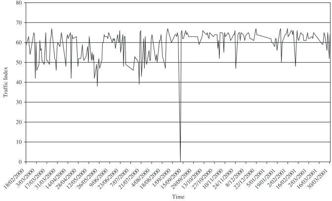
The data set is comprised of 58 time series, each containing 232 observations. These data-are sampled from a continuous data-generating process and obtained daily at 7 a.m. Australian Eastern Standard Time weekdays from 18 February 2000 to 3 March 2001. A representative specimen of these data is shown in Figure 1. These data oscillate between zero and 100 and appear to exhibit charac-teristics typical of stationary series. Another feature, common to many series in the data set, is the presence of occasional downward spikes. Spikes indicate high congestion and, depending on the

1_{The Internet Traffic Report URL is http://www.internettrafficreport.com/index.html.} 0 10 20 30 40 50 60 70 80

18/02/20003/03/200017/03/200031/03/200014/04/200028/04/200012/05/200026/05/20009/06/200023/06/20007/07 /2000

21/0 7/2000

4/08/2000₁₈/08/20001/09 /2000 15/0 9/2000 29/0 9/2000 13/10/200027/10/ 2000 10/11/200024/11/200

0 8/12/2000_22/12

/2000 5/01/2001_19/01/2

001 2/02/2001_16/02/20012/03/2

001 16/03/200 1 30/03/ 200 1 Time Traffic Index

Figure 1. Japan dm-gw1.kddnet.ad.jp

motivation for generating forecasts, can be treated as outliers that are atypical or incorporated in the model as infrequent but important characteristics of the data-generating process.

Summary statistics indicate the frequency of the downward spikes with 27 of the 58 routers report-ing at least one minimum value below the 25th percentile. Sampled regions include Australia, East Asia, Israel, North America, Russia, South America and Western Europe. Regions not included are Africa, Antarctica and most of the Middle East. The Denver denver-br2.bbnplanet.net router is recorded as providing the fastest response, while AOL1 pop1-dtc.atdn.net has the lowest response time. On average, the Perth1 opera.iinet.net.au router consistently provides the fastest response. Yahoo fe3-0.cr3.SNV.globalcenter.net typically records the slowest response.2

The sample average coefficient of variation is 6.3 and the corresponding standard deviation is 1.8.

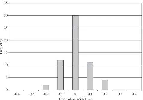
Following Fildes (1992), the frequency of outliers, strength of trend, degree of randomness and seasonality are analysed. The results are shown in Figures 2 to 5. An observation Xtis treated as an outlier when either Xt<Lx-1.5(Ux-L) or Xt>Lx+1.5(Ux-Lx), where Lxdenotes the lower quar-tile and Ux the upper quartile. The strength of trend is measured by the correlation between series (with outliers removed) and a time trend, with the absolute value of the trend indicating its strength. Randomness is measured by estimating the regression:

(1)

where X¢tdenotes the series Xtwith outliers removed. measures the variation explained by the

model. High indicates low randomness, while low reveals high randomness. Deterministic seasonality is estimated by regressing the series on an intercept and dummy variables which equal one when t =s, where tdenotes observation Xt’s position in time and s corresponds to the frequency of the seasonality. For example, to test the hypothesis that Mondays are statistically different to band-width capacity for the rest of the week, t = {1, 2, 3, 4, 5, . . . , T}, s ={1, 5, 10, 15, . . . , T} and dummy variable DMonday =0 for t = s, zero otherwise.

Figure 2 reveals half the series contain between 1% and 5% outliers. In percentage terms these data appear slightly more heterogeneous than Fildes’ (1992) telecommunications data. Figure 3 shows that these data are generally uncorrelated with time. This contrasts with Fildes, where the data exhibit strong negative trends. Moreover, histograms contained in Figures 3 and 4 reveal that vari-ation in these data presents a high degree of randomness with little serial correlvari-ation.

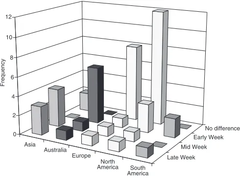
Finally, Figure 5 presents some evidence of regularity in weekly capacity variation aggregated by region. There appear regular dips occurring on different days across regions. Typically, Asia experi-ences lower traffic volumes from Wednesday through Friday, while most Australian routers have excess capacity from Monday through Tuesday. Conversely, Europe and North America experience a smoother traffic flow—perhaps due to more sophisticated capacity pricing and network manage-ment systems. Finally, South American Internet traffic variation is tied to particular routers.

The regressions are also conducted to test for regularity of both weekly and monthly traffic pat-terns. Weekly variation is not apparent, with only six routers reporting regular spikes across weeks. Surprisingly, given the short time series, substantial monthly variation was found for 95% of sampled routers.3

Although the sustained increase in traffic is too haphazard across routers to reveal a

cycli-R2 R2

R2

¢ = + + ¢ +- ¢ +- ¢

-Xt a bt d1Xt1 d2Xt 2 d3Xt 3

2_{Time-of-day and scale-of-demand effects may impact on router performance. For example, the Perth router services a small}

market and is likely to have relatively low congestion early in the morning, while in real time, the Yahoo router may be at peak demand in the mid-to-late afternoon.

0 1 2 3 4 5 6 7 8 9 10

0 1 2 3 4 5 6 7 8 9 10 11 12 13 14 15 16 17 18 19 Proportion of Outlying Observation (%)

Frequency

Figure 2. Outlier frequency

0 5 10 15 20 25 30 35

-0.4 -0.3 -0.2 -0.1 0 0.1 0.2 0.3 0.4 Correlation With Time

Frequency

Figure 3. Strength of linear trend

FORECAST MODELS AND ACCURACY MEASURES

Forecast models considered here are univariate ARARMA, ARMA, Filtered Trend, Holt, Holt-D exponential smoothing and Robust Trend against a benchmark Random Walk model. With the excep-tion of Filtered Trend, these forecast methods have been shown to be reliable by Fildes (1992), Makridakis et al. (1993), Fildes et al. (1998) and Makridakis and Hibon (2000), and consistently perform well in the M-competition. Implicit in these analyses, however, is that the majority of data included in the M-competition are non-stationary, while data analysed here are stationary. Given this

0 2 4 6 8 10 12 14 16 18

-0.02 -0.01 0.00 0.01 0.02 0.03 0.04 0.05 0.06 0.07 Adjusted R Squared

Frequency

Figure 4. Variation explained by linear/AR

No difference Early Week Mid Week Late Week Asia

Australia Europe

North America South

America 0

2 4 6 8 10 12

Frequency

Asia Australia Europe North America South America

fundamental difference in assumption, some of the forecast techniques are modified to avoid prob-lems associated with over-differencing. For example, the ARMA method is applied rather than ARIMA. ARARMA explicitly questions the practice of differencing to achieve stationarity and has an advantage of utilizing information contained in these data, normally lost when differencing. Moreover, the approach outlined in Parzen (1982) contains a method of determining when it is appro-priate to apply the AR filter, hence the method is adopted intact. Filtered Trend is simple extrapola-tion based on a regression of a series on a deterministic time trend after outliers have been removed. Holt and Holt-D methods provide adaptable alternatives to Filtered Trend while also retaining the advantage of simplicity and reliability. However, to ensure the opportunity for accuracy is max-imized, the parameter is re-estimated for each new estimation period, as recommended in Fildes et al. (1998), rather than being held fixed. Robust Trend differences the data before calculating the sto-chastic trend. The perceived advantage in adopting this method is the outlier filter and its use of the median rather than mean in estimation, which may provide some advantage over the simple Random Walk extrapolation. Accordingly, for comparison, Random Walk is employed as the benchmark. When outliers do not bias estimation, Random Walk forecasts are difficult to improve on, given the reported properties of these data.

The choice of accuracy measures is guided by the recommendations of Armstrong and Collopy (1992). They argue that the Mean Absolute Percentage Error (MAPE), Median Absolute Percentage Error (MdAPE), % Better, Geometric Mean Relative Absolute Error (GMRAE) and Median Rela-tive Absolute Error (MdRAE) best assess forecast performance. Both GMRAE and MdRAE are Winsorized as recommended by Armstrong and Collopy. Mean square error measures are avoided since these statistics are scale-dependent and sensitive to outliers.

FORECASTS

To identify the most accurate forecasting methods, six sets of forecasts are created by dividing these data into estimation and forecast segments. The estimation period is shifted forward 10 observations post-estimation. The model is re-estimated on this sample, and so on. Each forecast method uses 117 observations to forecast over the next 60 observations.4

That is, the approach uses a rolling window beginning at the first observation and steps forward 10 days, re-estimating the forecasts over the next 117 observations. The approach provides 348 forecasts with an equal lead time of 60 periods per method to judge forecast performance. In evaluating the reliability of the alternative methods, forecasts are compared to post-sample data values. The number of forecast windows is maximized to offset the distortions created by outlying observations at the end of each estimation window.5

All forecast methods are estimated in SHAZAM utilizing automatic procedures. For example, ARMA is implemented by conducting a grid search of autoregressive moving average parameters with maximum lag length set to 10. The best performing model is deemed to be the one that scores the lowest Akaike Information Criterion statistic. The test for the long-memory filter in ARARMA (Parzen’s Err(t) statistic) is used to determine the filter’s lag length. The long-memory procedure is

4_{60-day forecasts are necessary due to the existence of standard capacity contracts.}

5_{The effects of distortions created by these data are complex. To simplify the analysis, a total of 24 zero observations are}

verified using the results from the illustrative example provided in Parzen (1982).6

In most cases, the model is determined to be short memory and is estimated as an unfiltered ARMA. In a portion of the cases deemed to be long memory the Err(t) statistic is less than zero. Analysis of the inter-national airline data used by Parzen along with simulated data shows that data with exponential trends always yield positive Err(t) statistics. By contrast, the Internet bandwidth data does not exhibit any trend. The explanation for negative Err(t) statistics is provided by examining the calculations for Err(t) and the long-memory coefficient (t), which are defined as:

(2)

(t) is the sample correlation coefficient between the current observation and its counterpart lagged

tperiods. SSQ(T) is the sum of squares for all observations in the estimation window and SSQ(T

-t) is the sum of squares for observations between one and the observation corresponding to T-t. In the Internet bandwidth data, the calculated sum of squares increases linearly as Tincreases. Thus, the rate of increase in the ratio SSQ(T)/SSQ(T-t) is greater than the rate of decline in (t) (as lag

tincreases), resulting in a calculated coefficient (t) that can at times be substantially greater than one. The magnitude of the coefficient dominates the calculated Err(t), resulting in a negative statis-tic. Rejection of negative Err(t) statistics results in estimation of short-memory ARMA models. This problem is indicative of the need to consider the underlying properties of the data prior to selecting specific forecast methods.

In general, selected models for both ARMA and ARARMA exhibit short lags (on average between one and four lags) and are, therefore, highly adaptive. Seventeen percent of ARARMA models cal-culated positive Err(t) statistics that are less than the critical value, resulting in estimates of (t) that range between 0.94 and 1.02. Holt, Holt-D and Robust Trend parameters are optimized for each esti-mation window and series.

Table I presents forecast accuracy results through average absolute error calculations. In general, Filtered Trend performed better than the other methods with Robust Trend the next best. ARARMA and Holt-D consistently performed worst. The ARARMA statistic is biased by 23% of forecast models with substantial forecast errors. In general, it appears that the poor performance of ARARMA is closely related to outliers near the end of some estimation windows in a number of series. Of these, 30% correspond to use of the long-memory filter. The poor performance of Holt-D is likely due to over-differencing. Although Robust Trend also differences these data, parameter estimates are often small in magnitude. Thus, forecast errors deteriorate gradually. The short-term good perfor-mance of ARMA provides some assurance that automatic procedures can model time series reason-ably well. In the longer term, ARMA overtakes Robust Trend, indicating that flexible estimation of adaptive methods may be better for longer horizons.

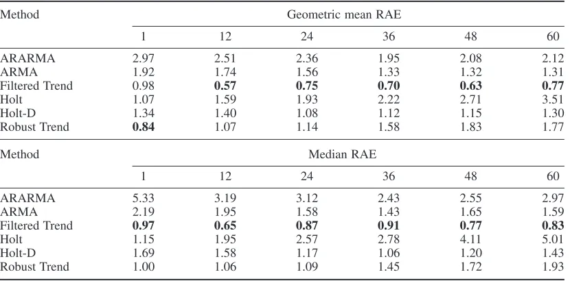
Further evaluation is reported in Table II, which presents the GMRAE and MdRAE forecast error measures. Both GMRAE and MdRAE compare each method to a ‘no-change’ benchmark forecast. A score of less than one indicates the forecast method is at least more reliable than the Random Walk benchmark. By these criteria Filtered Trend is the only method to consistently outperform the benchmark.

An important factor is accuracy variation over forecast horizons. M-competition results indicate some methods are better for short-term forecasts, while others perform better over longer horizon.

ˆ f ˆ f ˆ r ˆ r

ˆ ˆ ˆ

f t r t

t t f t

t t ( ) = ( ) ( ) -( ) ( ) = - ( ) -( ) ( ) - ( ) SSQ T SSQ T SSQ T

SSQ T SSQ

and Err 1 2

ˆ

f

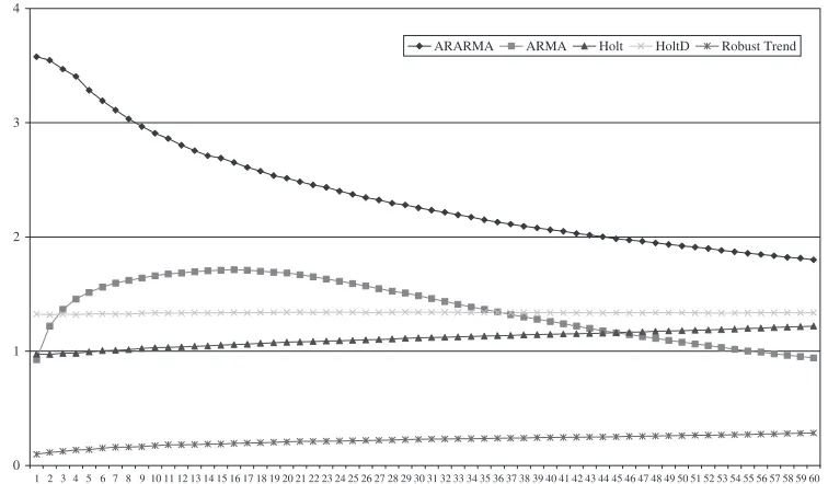
Figure 6 reports the cumulative forecast errors for the initial estimation window. As Figure 6 clearly shows, ARARMA is consistently worst. Interestingly, ARMA cumulative forecast accuracy improves as the forecast horizon lengthens, overtaking Holt and Holt-D. However, in terms of cumulative errors, none of the adaptive forecasts are particularly reliable.

Finally, Table III presents the proportion of better than Random Walk extrapolation forecasts. Results suggest that the best forecast method, Filtered Trend, has only a one in two chance of per-forming better than the naïve forecast. For relatively short horizons, Robust Trend outperforms the naïve benchmark. Robust Trend’s gradual deterioration in forecasts corresponds to its fixed trend direction, whereas ARMA and Holt are able to accommodate trend changes. Further, the results reaf-firm the relatively poor performance of ARARMA.

To sum, the results show that Internet bandwidth is most reliably forecast in the short run by deter-ministic trend methods. MAPE statistics show that Robust Trend tracks index values with an average

Table I. Mean absolute percentage error

Method Forecasting horizon

1 20 40 60 1–5 1–25 1–45 1–60

ARARMA 356 180 151 137 328 237 198 180

ARMA 15 53 13 14 151 159 116 94

Filtered Trend 8 10 15 5 13 18 8 8

Holt 17 67 36 50 100 110 116 122

Holt-D 136 134 132 132 133 134 134 134

Robust Trend 0 29 36 48 14 22 25 28

Note: Bold minimum MAPE statistic indicates the best performed method.

Table II. Geometric mean RAE and median RAE

Method Geometric mean RAE

1 12 24 36 48 60

ARARMA 2.97 2.51 2.36 1.95 2.08 2.12

ARMA 1.92 1.74 1.56 1.33 1.32 1.31

Filtered Trend 0.98 0.57 0.75 0.70 0.63 0.77

Holt 1.07 1.59 1.93 2.22 2.71 3.51

Holt-D 1.34 1.40 1.08 1.12 1.15 1.30

Robust Trend 0.84 1.07 1.14 1.58 1.83 1.77

Method Median RAE

1 12 24 36 48 60

ARARMA 5.33 3.19 3.12 2.43 2.55 2.97

ARMA 2.19 1.95 1.58 1.43 1.65 1.59

Filtered Trend 0.97 0.65 0.87 0.91 0.77 0.83

Holt 1.15 1.95 2.57 2.78 4.11 5.01

Holt-D 1.69 1.58 1.17 1.06 1.20 1.43

Robust Trend 1.00 1.06 1.09 1.45 1.72 1.93

variation of 28%, while ARMA’s average forecast provides a slight improvement for longer time horizons. The convergence in accuracy between ARMA and Filtered Trend suggests that ARMA may be useful in confirming the long forecasts generated by Filtered Trend. Finally, the inherent station-arity of these data may explain the failure of ARARMA and Holt-D forecast methods.

CONCLUSIONS

The study provides further evidence as to the link between data characteristics and forecast accu-racy for specific univariate extrapolation methods. Forecast techniques employed here are

extrapo-0 1 2 3 4

1 2 3 4 5 6 7 8 9 10 11 12 13 14 15 16 17 18 19 20 21 22 23 24 25 26 27 28 29 30 31 32 33 34 35 36 37 38 39 40 41 42 43 44 45 46 47 48 49 50 51 52 53 54 55 56 57 58 59 60 ARARMA ARMA Holt HoltD Robust Trend

Figure 6. Cumulative mean absolute percentage error

Table III. Percent better

Method Forecast horizon

1 6 12 18 24 30 36 42 48 54 60

ARARMA 19 20 19 16 18 17 20 18 19 21 21

ARMA 32 44 39 35 46 41 44 38 35 41 48

Filtered Trend 47 53 62 53 51 41 53 55 59 47 56

Holt 49 40 32 29 27 23 24 20 18 14 14

Holt-D 44 49 40 47 52 47 53 44 53 48 46

Robust Trend 51 53 44 40 42 34 34 31 30 27 29

lation methods that perform well in the M-competition and are easily implemented. In evaluating methods, a single data series is utilized to facilitate the analysis of forecast performance, conditional on the properties of these data. Analysis of summary statistics reveals that bandwidth data exhibit considerably less structure than telecommunications data as reported by Fildes (1992) and M-competition data (Fildes et al., 1998). As a result, the univariate extrapolation methods perform poorly when compared to previous studies. This outcome is not surprising as univariate extrapola-tion methods are intended to exploit data regularities, such as autocorrelaextrapola-tion and trend direcextrapola-tion, generally not present in bandwidth data. Study findings highlight the need to better understand the data characteristics, prior to forecasting. In particular, the high degree of randomness and the pres-ence of outliers are responsible for the performance of Filtered Trend and Robust Trend in relation to the other forecast methods. Finally, future research directed at developing a consistent approach to data classification may provide further useful insights into the optimal selection of forecast method.

ACKNOWLEDGEMENTS

We thank Jim Alleman, Robert Fildes and two anonymous referees for helpful comments. Coble-Neal benefited greatly from a presentation by J. Scott Armstrong delivered at the ICFC 2000 Con-ference in Seattle, Washington, September 2000. The usual disclaimer applies.

REFERENCES

Armstrong JS, Collopy F. 1992. Error measures for generalizing about forecast methods: empirical comparisons.

International Journal of Forecasting8: 69–80.

Clements MP, Hendry DF. 2001. Explaining the results of the M3 forecasting competition. International Journal of Forecasting17: 537–584.

Fildes R. 1992. The evaluation of extrapolative forecasting methods. International Journal of Forecasting8: 81–98.

Fildes R, Ord JK. 2002. Forecasting competitions—their role in improving forecasting practice and research. In

A Companion to Economic Forecasting, Clements M, Hendry D (eds). Blackwell: Oxford.

Fildes R, Hibon M, Makridakis S, Meade N. 1998. Generalising about univariate forecasting methods: further empirical evidence. International Journal of Forecasting14: 339–358.

Makridakis S, Hibon M. 1979. Accuracy of forecasting: an empirical investigation. Journal of the Royal Statisti-cal Society, Series A142(Part 2): 97–145.

Makridakis S, Hibon M. 2000. The M3-competition: results, conclusions and implications. International Journal of Forecasting16: 451–476.

Makridakis S, Anderson A, Carbone R, Fildes R, Hibon M, Lewandowski R, Newton J, Parzen E, Winkler R. 1982. The accuracy of extrapolation (time series) methods: results of a forecasting competition. Journal of Fore-casting1: 111–153.

Makridakis S, Chatfield C, Hibon M, Lawrence M, Mills T, Ord K, Simmons LF. 1993. The M-2 competition: a real-time judgmentally based forecasting study. International Journal of Forecasting9: 5–23.

Opinix. 2001. Internet Traffic Report. http://www.internettrafficreport.com.

Parzen E. 1982. ARARMA models for time series analysis and forecasting. Journal of Forecasting1: 67–82.

Authors’ biographies:

which supports CEEM, has come from industry, government and the Australian Research Council. He is a mutiple recipient of the CBS Researcher of the Year, Article of the Year and Book of the year awards. Gary is Editor of the Edward Elgar series, the International Handbook of Telecommunications Economics, Volumes I–III. He is a Member of the Board of Management of the International Telecommunications Society, and a Member of the Edi-torial Board of the Journal of Media Economics.

Grant Coble-Neal was Research Associate at the Communication Economics and Electronic Markets Research Centre (CEEM), Curtin University of Technology, Australia from 1999 to 2003. During that time Grant co-authored several articles with Gary Madden analyzing various aspects of the telecommunications industry. Prior to joining CEEM, Grant worked for several government agencies. He is currently attempting to complete his doc-toral studies.

Authors’ addresses: