Bilexical Embeddings for Quality Estimation

(1)

Bilexical Embeddings for Quality Estimation

Fr´ed´eric Blain, Carolina Scarton and Lucia Specia Department of Computer Science

University of Sheffield, UK

{f.blain, c.scarton, l.specia_}@sheffield.ac.uk

Abstract

This paper describes the SHEF submis-sions for the three sub-tasks of the Qual-ity Estimation shared task of WMT17, namely: (i) a word-level prediction sys-tem using bilexical embeddings, (ii) a phrase-level labelling approach based on the word-level predictions, (iii) a sentence-level prediction system using word em-beddings and handcrafted baseline fea-tures. Results are promising for the sentence-level approach, but still very pre-liminary for the other two levels.

1 Introduction

Quality Estimation (QE) allows the evaluation of Machine Translation (MT) when reference trans-lations are not available. It can be used in vari-ous ways such as in post-editing (PE) to predict whether or not an automatically generated sen-tence is worth publishing, editing or it should be retranslated manually. Word-level predictions can be helpful by highlighting words that cannot be relied upon or should be fixed by post-editors. More recently, QE at phrase-level has emerged as a way of using quality predictions at decoding time in phrase-based Statistical MT (SMT) sys-tems to guide the decoder such as to keep phrases which are predicted as good, and conversely to dis-card those which are predicted as bad (Logacheva,

2017).

QE models are built based on a list of features along with a Machine Learning algorithm for ei-ther regression or classification. These features are usually extracted from the source and target texts or from the MT system that generated the transla-tions. Shah et al.(2015) introduced a new set of features extracted using an unsupervised approach with the use of neural network: continuous-space

language model features and word embeddings features.

In our contribution this year we investigate whether we can go beyond engineered features by learning bilexical operators over distributional representations of words in source-target text pairs. Considering the MT pipeline as a noisy black-box, our motivation is to be able to build QE models to predict if information encoded in the source sentence is preserved in the target sentence after translation.

2 Bilinear Model

Madhyastha et al. (2014) propose to use word-level embeddings to predict the strength of differ-ent types of lexical relationships between a pair of words, such as head-modifier relations between noun-adjective pairs. They designed a supervised framework for learning bilexical operators over distributional representations, based on learning bilinear forms W. We adapted their method to predict the strength of relationship between source and target words. This problem is formulated as a log-bilinear model, parametrized with W as fol-lows:

Pr(t|s;W) = exp

n

φ(t)>W φ(s)o

X

t0_∈T

expnφ(t0)>W φ(s)o (1)

where φ denotes the word embeddings of any given word in a vocabulary V.The source words s and target words t are respectively taken from subspacesS ⊆ V andT ⊆ V.

In essence, the problem can be reduced to first obtaining the corresponding word embeddings of the vocabularies of both source and target sen-tences using a substantially large monolingual cor-pus for each of the two languages, followed by us-ing the bilinear model to estimateW.W is learned

(2)

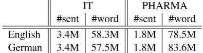
IT PHARMA #sent #word #sent #word English 3.4M 58.3M 1.8M 78.5M German 3.4M 57.5M 1.8M 83.6M

Table 1: Statistics of the in-domain data used to train our embeddings.

using the source-target word alignment by mini-mizing the negative log-likelihood using a`2

reg-ularized objective as:

L(W) =₋X s,t

log(P r(t_|s;W)) +λ_kW_k2 (2)

whereλis the constant that controls the capacity ofW with gradient descent-based optimization.

We explore this approach for both word and phrase-level QE. For training, we rely on both the word-alignments and the gold QE labels (i.e. the

OK/BAD labels). The former gives us the source-target pairs, and the latter whether this pair is valid or not. Our assumption is that this approach should be able to predict whether or not a word in the target language (MT output) is correct by ex-ploring the strength of the linguistic relation with the source word it is generated from.

3 Experimental Settings 3.1 Data and Gold labels

Each QE shared task has two datasets: English→German segments on the IT do-main (with 23,000 sentences for training, 1,000 for development and 2,000 for test), and German→English segments on the Pharmaceuti-cal domain (with 25,000 sentences for training, 1,000 for development and 2,000 for test). The same data is used for all three tasks: word, phrase and sentence-level prediction.

For the word-level task, each token of the MT is annotated with OK or BAD labels. For the phrase-level task, phrases are segmented as given by an SMT decoder and also annotated with OK

orBADlabels. Finally, for the sentence-level task, the quality label is a Human-Targeted Error Rate (HTER) score (Snover et al.,2009).

3.2 Word Embeddings

Word embeddings were used in our submissions for the three tasks. We trained in-domain skip-gram embeddings on the in-domain data shown in

Table1using FastText1₍_{Bojanowski et al.}_,₂₀₁₆₎ with 300 dimensions and learning rate set to 0.025. The default training settings are otherwise used. The in-domain data is the same as that used to train the SMT system that produced the translations in the QE datasets, as made available by the task or-ganizers.

For the word and phrase-level tasks, we used our word embeddings to obtain a word vector rep-resentation of 300 dimensions for each word of both the training and development sets. For the sentence-level task, the word embeddings are av-eraged for each sentence, as previously applied in (Scarton et al.,2016).

3.3 Tool

To learn to predict the labels for the word-level task, we used BMAPS2, the toolkit implementing

the method in (Madhyastha et al., 2014) along with the word alignments provided by the organiz-ers (as produced by the SMT system). BMAPSis

used to learn the bilexical operators between both source and target embeddings. The tool relies on three matrices corresponding to the source and tar-get vocabularies of the training data, and a third matrix representing the word-level lexical relation between them. This matrix is built from the word-level alignments and the gold labels to indicate which lexical items form a pair, and whether their lexical relation is OKor BAD (i.e. if two lexical items are aligned and labelled as OK, their inter-section in the third matrix is set to1,0otherwise). By default, the model is trained over 100 it-erations with the l2 norm as regularizer, and

us-ing theforward-backward splittingalgorithm (FO-BOS) (Duchi and Singer, 2009) as optimization scheme (lc= 0.1,tau= 0.1).

3.4 Evaluation

We used the official task metrics to evaluate our re-sults. For the word and phrase-level tasks, the met-rics areF1-BAD andF1-OK which correspond to

theF1scores on bothBADandOKlabels, andF1

-multi which is the product of the two formers. For the sentence-level task, the metrics for scoring are Pearson’s correlation (primary metric), Mean Av-erage Error (MAE) and Root Mean Squared Error (RMSE), and for ranking, Spearman’s rank corre-lation (primary metric) and DeltaAvg.

1_{https://github.com/facebookresearch/}

fastText

[image:2.595.76.285.63.118.2]

(3)

4 Results

4.1 Word-level QE prediction (Task 2) We investigate different context windows to build our lexical representations, ranging from a wide window considering all sentence-level context, to a much narrower approach representing each word individually:

• Full context: each word is associated with

its left and right context to capture the exact distributional features of the specific context in which this lexical item occurs. A lexical item is thus a 900-dimensional word vector represented by the tuple < emblef t, embcur, embright>, whereemblef t

andembrightare the averaged embeddings of

the left/right contexts and embcur the word

representation of the current word. Here our assumption is that a lexical item would repre-sent a word within its context and at its posi-tion in the sentence, therefore if the word ap-pears twice in the sentence, it would be rep-resented by two different lexical items.

• Surrounding context: instead of consider-ing all the left and right context of the cur-rent word, we limit ourselves to the two sur-rounding words. This allows for a model that is as generic as possible while still consider-ing two distributional features correspondconsider-ing to two different lexical items. Here the as-sumption is the same as before, the lexical item which represents a word is the same but only considering a window of one word on the left/right to computeemblef t/embright.

• Unigram: we use only the embeddings of

the current word without considering any sur-rounding context. By doing so, we fully rely on the embeddings and the way they are trained (skipgram). In this case, the lexical item is a single word representation of 300 dimensions.

For each context we investigate two variants: with and without the use of the gold labels in or-der to demonstrate the capacity of our approach to learn how to discriminate the valid lexical pairs from the others.

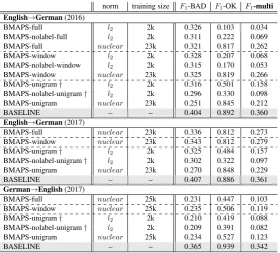
Discussion The results of our approach for the word-level task are given in Table2. We report the results of our official submissions to the task (†)

along with additional experiments we conducted after the task deadline. They are both compared with the official baseline of Task 2.

Our first observation is the overall low perfor-mance of our approach compared to the official baseline. However, we found very encouraging the results of our additional experiments compared to those of the systems submitted. The revised training procedure significantly improved the per-formance in terms ofF1-OK for all three contexts

types, resulting in a boost in theF1-multi scores.

To better understand the gap between our offi-cial and additional results, it is important to men-tion the technical constraints we faced perform-ing the task with BMAPS for the official

submis-sion. In its current implementation, BMAPSrelies

on non-sparse matrices which in our case lead to a heavy memory print, since the source and the target matrices contain vector representations for each word in the corpus. Therefore, to be able to run BMAPSon our servers we were limited to use

up to 2,000 sentences (about 9% of the training corpus) as training instances. This certainly had a significant impact on the performance of the mod-els.

To tackle this constraint we later opted for a mini-batch training approach: we divided the training corpus into batches of 500 sentences, the training for each batch starting from the results from the training with the previous one. By doing so we are able to use all the training data. How-ever, in BMAPS the size of the dev set (in terms

of words from which the matrices are built) has to be smaller than that of the training set. There-fore, by using mini-batches we had to reduce our dev set. We selected for the dev set 250 sentences with the highest number ofOK labels in order to boost performance for this class. We also refined our training parameters by switching to the nuclear norm (which is expected to converge faster when restricting the training size (Madhyastha et al.,

2014)). Finally, we empirically identified the best values for the two main parameters (namelylcand tau) for different context types: for both the full and surrounding context, we used lc = 0.1 and

tau = 0.001, while for the unigram approach we

usedlc= 0.1andtau= 0.01.

(4)

be-norm training size F1-BAD F1-OK F1-multi

English→German(2016)

BMAPS-full l2 2k 0.326 0.103 0.034

BMAPS-nolabel-full l2 2k 0.311 0.222 0.069

BMAPS-full nuclear 23k 0.321 0.817 0.262

BMAPS-window l2 2k 0.328 0.207 0.068

BMAPS-nolabel-window l2 2k 0.315 0.170 0.053

BMAPS-window nuclear 23k 0.325 0.819 0.266

BMAPS-unigram† l2 2k 0.316 0.501 0.158

BMAPS-nolabel-unigram† l2 2k 0.296 0.330 0.098

BMAPS-unigram nuclear 23k 0.251 0.845 0.212

BASELINE – – 0.404 0.892 0.360

BMAPS-unigram† l2 2k 0.325 0.484 0.157

BASELINE – – 0.407 0.886 0.361

German→English(2017)

BMAPS-unigram† l2 2k 0.210 0.419 0.088

[image:4.595.160.441.61.314.2]

BASELINE – – 0.365 0.939 0.342

Table 2: Results of our word-level predictions. †denotes our official submissions to the task using the

l2 norm and single training set of 2k sentences. The other figures are obtained with mini-batch training

using 500 sentences at the time. In grey are the results of the official baseline of the task.

tween the three types of context: while unigram was the best performing when limited to 2k train-ing instances only, the exact opposite was found when using the full training set with better F1-*

scores when the context in which the word occurs is employed. Furthermore, we note a small advan-tage for the window context over the full context in both language pairs. We believe this means that considering the surrounding context could better help in a situation where a word would appear twice in the same sentence but should be labelled differently.

Overall, these results are encouraging and we aim to pursue further investigations towards im-proving this approach for the task of word-level QE.

4.2 Phrase-level QE labelling (Task 3)

While we could have chosen to predict phrase-level QE labels similarly to our word-phrase-level predic-tions, we opted for generating phrase-level labels from word-level labels following the labelling ap-proaches described inBlain et al.(2016):

• Optimistic: if half or more of words have a labelOK, the phrase has the labelOK (major-ity labelling).

• Pessimistic: if 30% words or more have a

labelBAD, the phrase has the labelBAD.

• Super-pessimistic:if any word in the phrase has a labelBAD, the whole phrase has the la-belBAD.

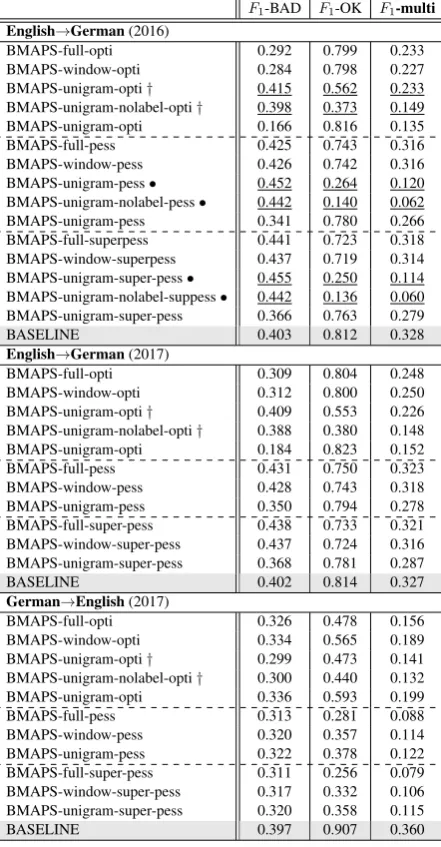
Discussion The results of these three phrase-level labelling strategies based upon our word-level predictions are given in Table 3. We re-port the results of our official submissions to the task (†) along with additional experiments we con-ducted after the task deadline. These are compared with the official baseline for Task 3.

First, similarly to the word-level task, the per-formance at phrase-level improved with the addi-tional experiments, which was expected since the labelling directly follows from the word-level pre-dictions. Second, while we originally observed better labelling performance using the optimistic approach on test.2016 (see underlined numbers), we now observe betterF1-* scores with both

pes-simistic approaches for en→de. One can also

ob-serve comparable performance for en→de when the surrounding context is used: the difference in terms ofF1-* scores between the full and window

(5)

la-F1-BAD F1-OK F1-multi

BMAPS-full-opti 0.292 0.799 0.233

BMAPS-window-opti 0.284 0.798 0.227 BMAPS-unigram-opti† 0.415 0.562 0.233 BMAPS-unigram-nolabel-opti† 0.398 0.373 0.149 BMAPS-unigram-opti 0.166 0.816 0.135

BMAPS-full-pess 0.425 0.743 0.316

BMAPS-window-pess 0.426 0.742 0.316 BMAPS-unigram-pess• 0.452 0.264 0.120 BMAPS-unigram-nolabel-pess• 0.442 0.140 0.062 BMAPS-unigram-pess 0.341 0.780 0.266 BMAPS-full-superpess 0.441 0.723 0.318 BMAPS-window-superpess 0.437 0.719 0.314 BMAPS-unigram-super-pess• 0.455 0.250 0.114 BMAPS-unigram-nolabel-suppess• 0.442 0.136 0.060 BMAPS-unigram-super-pess 0.366 0.763 0.279

BASELINE 0.403 0.812 0.328

BMAPS-full-opti 0.309 0.804 0.248

BMAPS-full-pess 0.431 0.750 0.323

BMAPS-window-pess 0.428 0.743 0.318 BMAPS-unigram-pess 0.350 0.794 0.278 BMAPS-full-super-pess 0.438 0.733 0.321 BMAPS-window-super-pess 0.437 0.724 0.316 BMAPS-unigram-super-pess 0.368 0.781 0.287

BASELINE 0.402 0.814 0.327

BMAPS-full-opti 0.326 0.478 0.156

BMAPS-full-pess 0.313 0.281 0.088

BMAPS-window-pess 0.320 0.357 0.114 BMAPS-unigram-pess 0.322 0.378 0.122 BMAPS-full-super-pess 0.311 0.256 0.079 BMAPS-window-super-pess 0.317 0.332 0.106 BMAPS-unigram-super-pess 0.320 0.358 0.115

BASELINE 0.397 0.907 0.360

Table 3: Results of the phrase-level labelling strategies based upon our word-level QE predic-tions.†denotes our official submissions to the task and•the results of the other two labelling

strate-gies, both using our official submissions to Task 2. The other figures are obtained with the updated word predictions from Task 2 resulting of the full batch training. In grey are the results of the official baseline of the task.

belling based on word prediction using the entire sentence as context.

4.3 Sentence-level QE prediction (Task 1) For the sentence-level task we followed a sim-ple approach, which had been previously applied by Scarton et al. (2016) for document-level QE. The idea was to combine word embeddings with handcrafted features.

However, whilstScarton et al.(2016) have used

Scoring Ranking

Pearson’sr MAE Spearman’sρ DeltaAvg English→German(2016)

QUEST-EMB 0.50 0.12 0.53 9.02

BASELINE 0.40 0.13 0.44 7.42

QUEST-EMB 0.50 0.13 0.51 8.96

BASELINE 0.40 0.14 0.43 7.45

QUEST-EMB 0.56 0.12 0.56 8.79

[image:5.595.75.296.63.487.2]

BASELINE 0.44 0.13 0.45 6.81

Table 4: Results of QUEST-EMB in the sentence-level QE task. In grey are the results of the official baseline of the task.

word embeddings trained on general purpose data, our embeddings are trained over in-domain data, as previously described. Word embeddings were averaged at sentence level in order to have a single vector representing each sentence. We then con-catenated source and target in-domain embeddings with the 17 sentence-level baseline features pro-vided by the organisers. An SVM regressor was used to train our QE model with hyper-parameters optimized via grid-search. For that we used the learning module available at QuEst++ toolkit (Specia et al.,2015).

Although the sentence-level experiment is dif-ferent from the approach applied for word and phrase-level tasks, our aim was to test the usabil-ity of the in-domain word embeddings. Our results are compared with the official baseline.

Discussion The results of our sentence-level predictions are given in Table 4. Although the approach is rather simplistic, it achieves consid-erably good results by outperforming the baseline system and several other systems that participated in the shared task. For German→English, our

sys-tem performed seventh out of 13 in the scoring

task. For English→German, it performed eighth out of13. Table4shows the results of our systems

(called QUEST-EMB) for the different language pairs and for both scoring and ranking tasks. We also show the results of the baseline systems for comparison.

5 Conclusions

[image:5.595.310.524.64.170.2]

(6)

a bilinear model. Due to limitations regarding the experimental settings of the tool used for the offi-cial submissions, it is difficult to conclude whether or not our approach is suitable for the task of QE. In follow up experiments with different training strategies, the results proved substantially better and much more promising, albeit still behind the official baseline. This is particularly encouraging considering that the approach only relies on word embeddings and word alignment information. We plan to further experiment with it and identify pos-sible improvements in BMAPS that could lead to

better performance.

It is also worth emphasizing that the approach employed for the sentence-level task is not directly comparable to the approach used for the other tasks; they only share the embeddings trained us-ing in-domain data. However, we can conclude that the domain embeddings encode useful in-formation for all tasks.

Acknowledgments

The authors would like to thank Pranava S. Mad-hyastha for his support regarding the use of BMAPS. This work was supported by the QT21

project (H2020 No. 645452).

References

Fr´ed´eric Blain, Varvara Logacheva, and Lucia Specia. 2016. Phrase level segmentation and labelling of machine translation errors. In Tenth International

Conference on Language Resources and Evaluation.

Portoroz, Slovenia, pages 2240–2245.

Piotr Bojanowski, Edouard Grave, Armand Joulin, and Tomas Mikolov. 2016. Enriching word vec-tors with subword information. arXiv preprint

arXiv:1607.04606.

John Duchi and Yoram Singer. 2009. Efficient on-line and batch learning using forward backward splitting. Journal of Machine Learning Research

10(Dec):2899–2934.

Varvara Logacheva. 2017. Human Feedback in

Statis-tical Machine Translation. Ph.D. thesis, The

Uni-versity of Sheffield.

Pranava Swaroop Madhyastha, Xavier Carreras, and Ariadna Quattoni. 2014. Learning task-specific bilexical embeddings. In Proceedings the 25th International Conference on

Computa-tional Linguistics. Dublin, Ireland, pages 161–171.

http://www.aclweb.org/anthology/C14-1017.

Carolina Scarton, Daniel Beck, Kashif Shah, Karin Sim Smith, and Lucia Specia. 2016. Word embed-dings and discourse information for Quality Estima-tion. InProceedings of the First Conference on

Ma-chine Translation. Berlin, Germany, pages 831–837.

Kashif Shah, Varvara Logacheva, Gustavo Paetzold, Fr´ed´eric Blain, Daniel Beck, Fethi Bougares, and Lucia Specia. 2015. Shef-nn: Translation quality estimation with neural networks. InProceedings of the Tenth Workshop on Statistical Machine Transla-tion. pages 342–347.

Matthew Snover, Nitin Madnani, Bonnie J. Dorr, and Richard Schwartz. 2009. Fluency, Adequacy, or HTER? Exploring Different Human Judgments with a Tunable MT Metric. In The Fourth Workshop

on Statistical Machine Translation. Athens, Greece,

pages 259–268.

Lucia Specia, Gustavo Paetzold, and Carolina Scarton. 2015.Multi-level translation quality prediction with quest++. InProceedings of ACL-IJCNLP 2015

Sys-tem Demonstrations. Association for Computational