warwick.ac.uk/lib-publications
Original citation:
Liberini, Federica, Redoano, Michela and Proto, Eugenio. (2017) Happy voters. Journal of
Public Economics, 146 . pp. 41-57.
Permanent WRAP URL:
http://wrap.warwick.ac.uk/84425
Copyright and reuse:
The Warwick Research Archive Portal (WRAP) makes this work by researchers of the
University of Warwick available open access under the following conditions. Copyright ©
and all moral rights to the version of the paper presented here belong to the individual
author(s) and/or other copyright owners. To the extent reasonable and practicable the
material made available in WRAP has been checked for eligibility before being made
available.
Copies of full items can be used for personal research or study, educational, or not-for-profit
purposes without prior permission or charge. Provided that the authors, title and full
bibliographic details are credited, a hyperlink and/or URL is given for the original metadata
page and the content is not changed in any way.
Publisher’s statement:
© 2017, Elsevier. Licensed under the Creative Commons
Attribution-NonCommercial-NoDerivatives 4.0 International
http://creativecommons.org/licenses/by-nc-nd/4.0/
A note on versions:
The version presented here may differ from the published version or, version of record, if
you wish to cite this item you are advised to consult the publisher’s version. Please see the
‘permanent WRAP URL’ above for details on accessing the published version and note that
access may require a subscription.
Happy Voters
IFederica Liberini
ETH, Z¨urich
Michela Redoano1
University of Warwick
Eugenio Proto
University of Warwick and IZA
Abstract
Empirical models of retrospective voting primarily employ standard monetary and financial
indicators to proxy for voters’ utility and to explain voters’ behavior. We show that
sub-jective well-being explains variation in voting intention that goes beyond what is captured
by these monetary and financial indicators. For example, individuals who are satisfied with
their life are 1.6% more likely to support the incumbent; by contrast, a 10% increase in
family income leads to a 0.18% increase in an individual’s support of the incumbent. We
use difference-in-differences analysis to identify how voter intention is affected by a negative
shock to well-being: the death of a spouse. Individuals who experience the death of a spouse
are around 10% less likely than those in the control group to support the incumbent. The
results hold even if elected officials’ policies (health care, social welfare) cannot reasonably
be blamed for the death.
Keywords: Subjective Well-being, Happiness, Retrospective Voting.
JEL CLASSIFICATION: H1, D6, D0, D1.
IAcknowledgements: We would like to thank Stefano DellaVigna, Jan-Emanuel DeNeve, Peter Hammond,
Alan Manning, Richard Layard, Andrew Oswald, Daniel Sgroi, Fabian Waldinger, for very useful discussions and suggestions and participants of the Dr@w Forum (Warwick), Public Economic Conference (Exeter), LSE Wellbeing Seminar, International Institute of Public Finance Seminar (Lugano), Public Economic Theory Conference (Seattle). Financial support from CAGE (Warwick) is gratefully acknowledged.
1Address for correspondence; Department of Economics, Warwick University, Coventry, CV4 7 AL,
1. Introduction
There is a wide consensus in economics and political science that past outcomes affect
current voting decisions. In particular, according to the retrospective voting literature (e.g.,
Kramer, 1971; Fiorina, 1978, 1981; Kinder and Kiewiet, 1981; Markus, 1988; Lewis-Beck,
5
1990), voters compare past levels of utility and evaluate diagnostic information, such as
macroeconomic trends and personal financial circumstances, to re-elect good incumbents
and punish those who are believed to be corrupt, incompetent, or ineffective. At the same
time the political business cycle literature (e.g. Frey and Lau, 1968; Nordhaus, 1975) has
shown that policymakers, aware of this mechanism, regularly attempt to boost their chances
10
of staying in power by maximizing voters’ utility just before each election. The common
denominator of most of the empirical studies in these literatures is the use of financial and
economic indicators as proxies for voters’ utility.
More recently, the idea that policymakers should consider not only monetary and
fi-nancial indicators, but also rely on more comprehensive measures of well-being to inform
15
policies has become a subject of considerable debate among western policymakers and
schol-ars. Steps in this direction have been taken by the British and French governments as well
as by international organizations such as the World Bank, the European Commission, the
United Nations, and the OECD.2
This paper investigates whether subjective well-being (SWB) measures can be used to
20
proxy for utility, and explain the variation in voting intentions that goes beyond what is
captured by standard financial and economic indicators. In this respect, there is growing
consensus that indices of SWB constitute reasonably good proxies for utility. In particular
they can be understood as an application of experienced utility that – as discussed in
Kahneman and Thaler (1991) – is the pleasure derived from consumption. There is a
25
relatively old debate, mostly among psychologists, on whether individuals correctly recollect
their pleasure from past experiences (see Rabin, 1998, for review of this debate) and whether
individuals really make choices aimed to maximize their pleasure (e.g. Tversky and Griffin,
2For example, in 2008, the French government set up a Commission led by Joseph Stiglitz for the
1991; Hsee, 1999). In general, psychologists emphasize the existence of biases in the relation
between choice and predicted affective reactions. Recently Benjamin et al. (2012) test
30
explicitly in a lab setting if individuals tend to maximize SWB when choosing between
different scenarios; they show that this occurs in 80% of the cases. Furthermore, there are
several studies in economics using SWB indicators to infer the marginal rate of substitutions
between goods or state of the words under the implicit assumption of SWB being a proxy
for utility, see for example Di Tella, MacCulloch, and Oswald (2001), Benjamin et al. (2014)
35
and also Clark, Frijters, and Shields (2008) for a review of papers along these lines.
To address our question we introduce indicators of well-being as additional explanatory
variables in standard models of retrospective voting to serve as proxies for utility and to
explain individuals’ voting decisions. We use the well-being measures along with the
tradi-tionally used measures of financial economic conditions. We construct measures of voting
40
intentions and SWB using the British Household Panel Survey (BHPS), a rich database
started in 1991 containing information on over 10,000 British individuals on a yearly basis.
Consistent with the retrospective voting hypothesis, we find that SWB affects the
prob-ability of supporting the party of the Prime Minister together with and independently from
variables reporting improvement or worsening in family finances. Our estimates indicate that
45
individuals who are satisfied with their lives are 1.6% more likely to support the incumbent.
It is instructive to compare this figure with the one obtained from financial indicators: for
individuals who feel that their financial situation has improved (worsened) over time the
probability of supporting the incumbent is around 1.2% higher (lower); and an individual
whose family has experienced a 10% increase in family income is around 0.18% more likely
50
to support the incumbent party. Our findings suggest that both SWB and financial
po-sition indicators contribute to explaining voters’ behavior and both should be included as
regressors in the final econometric model.
Obvious concerns when exploring the relationship between voting and well-being are
reverse causality and omitted variable bias: the happiness of citizens with strong ideological
55
identities can be affected by an electoral success per se, rather than by the positive
out-comes of valid implemented policies, as Di Tella and MacCulloch (2005) have shown. We
address this concern in two different ways: (i) we analyze the responses of a sub-sample
of ideologically neutral individuals (i.e. those who do not have a priori party bias) whose
well-being should not be affected by the identity of the ruling party per se; and (ii) we
identify the effect of SWB on voting intentions by analyzing individuals’ responses to an
exogenous shock of (un)happiness. We consider these issues in turn.
Reverse causality between SWB and voting intentions can occur because some voters may
have ideological preferences for one party. Our idea is to replicate our estimations for the
subsample of respondents who are ideologically neutral (following the literature, we refer to
65
them asswingvoters henceforth). Selected questions asked in the BHPS allow us to identify
these individuals: our swing voters subsample covers about 30% of the full sample. SWB
measures remain very significant for this second set of estimations, but their magnitude is
much larger: swing voters who are satisfied with their life are 2.4% more likely to support
the incumbent. Furthermore, for the full sample, an increase of 1 unit in the reported life
70
satisfaction raises the probability of supporting the incumbent by 0.013 standard deviations,
while for the swing voter subsample this increment is nearly double. This result acquires
particular relevance in the context of the open debate on micro-targeting of floating voters
during election campaigns.
The second way we address the concern of identification is by analyzing variation in
75
respondents’ voting intentions due to a shock of SWB. We exploit the fact that some
re-spondents have experienced the death of their spouse during the period covered by the BHPS
.3 We treat this event as an exogenous variation of SWB. We use difference-in-differences
(DiD) analysis and propensity score matching to identify the effect on voting intention due
to this shock. We compare before- and after-the-shock changes in political support responses
80
of affected individuals to changes in political support responses of unaffected individuals.
This set-up not only provides a way to address concerns related to the identification of the
effect running from SWB to voting, but also allows us to analyze another important issue
still open in the literature: do voters punish or reward policymakers for events that are
largely independent from government’s actions? It is reasonable to think that the death
85
of a spouse is an event largely beyond government’s control, however confounding factors
can complicate the identification of the extent to which changes in wellbeing affect voting
intentions. For example, in some cases one could argue that the death of an individual
results from poor health care, for which the current government is ultimately accountable.
If this is the case, punishing the government is not an irrational behavior. We address this
90
3This event has been widely documented as having a deep, negative impact on the SWB of the surviving
point by exploiting the fact that in 1996 the Labour Party took over from the Conservative
Party in ruling the country. As a result, those individuals who became widows during the
Conservatives years should be unlikely to blame the government for the death of the partner
when a Labour government was in power.
We find that, in the two years following the death of a spouse, subjects in the treated
95
group are about 8% less likely to be pro-incumbent than individuals in the control group.
Interestingly, women seem to experience a sharper decline in SWB than men, and,
con-sistently with our hypothesis, women also show a stronger decline in incumbent support.
The different effect between men and women seems to be also in line with the evidence of a
gender gap in happiness, as highlighted by Stevenson and Wolfers (2009). Moreover, we find
100
evidence in support of the hypothesis that voters tend to blame the government for events
for which it is not generally responsible, by showing that the change of the party ruling the
country does not affect individuals’ attitudes towards the government.4
There is a related literature consistent with our conclusions. Achen and Bartels (2004)
show that voters are more likely to oust incumbents for the economic consequences of
nat-105
ural disasters. Healy, Malhotra, and Hyunjung Mo (2010) explore the electoral impact of
local college football games just before an election and find that a win in the ten days
be-fore Election Day causes the incumbent to receive an additional 1.6 percentage points. In
the same vein, Wolfers (2002) measures the extent to which voters in state gubernatorial
elections irrationally hold the state governor accountable for economic fluctuations that are
110
unrelated to his or her actions in office. More recently, Bagues and Esteve-Volart (2016),
considering the Spanish Christmas Lottery, find that incumbents receive significantly more
votes in lottery-winning provinces. Crucially, this literature does not analyze the role of
SWB in mediating voting intention. In addition, the literature uses aggregated data on
electoral results, which does not guarantee a connection between the exogenous event under
115
analysis and the individuals personally affected by it. A criticism usually directed to some
contributions in this literature is that exogenous shocks make voters more aware about the
quality of incumbent politicians (e.g. Ashworth and Bueno de Mesquita, 2016). Using SWB
indicators in our analysis suggests that more information cannot be the only explanation.
4Gurdal, Miller, and Rustichini (2013) suggest a rational explanation for this mechanism; they argue that
We find that government’s popularity mirrors the patterns of SWB, i.e. within three years
120
of a shock, an individual’s support for the government returns to the level indicated prior to
the occurrence of the shock. There is no particular reason to justify the fact that a better
informed voter “forgives” the incumbent once the negative shock is reabsorbed.
To the best of our knowledge, we are the first to directly analyze the effect of SWB
indicators on incumbent support. Several contributions have analyzed the effect of SWB on
125
political participation rather than voting decision (e.g., Dolan, Metcalfe, and Powdthavee,
2008; Killian, Schoen, and Dusso, 2008; Weitz-Shapiro and Winters, 2011; Flavin and Keane,
2012; Pacheco and Lange, 2010). These contributions indicate a positive link especially going
from SWB to participation.
A related literature looks at the relationship between partisanship and well-being;
no-130
tably, Di Tella and MacCulloch (2005) show that left-wing voters’ well-being is positively
affected by left-wing party victories and left-wing policy outcomes (like unemployment),
and the right-wing voters’ well-being, by right-wing electoral victories andright-wing
pol-icy outcomes (inflation targeting). Powdthavee and Oswald (2010, 2014) and Giuliano and
Spilimbergo (2014) show that exogenous shocks affect individuals’ political stances.
Follow-135
ing these contributions, we test the hypothesis that the effect on voting as the result of a
spouse’s death is different when the incumbent is left- or right-win. We do not find any
significant difference.
Finally, we would like to emphasize that one of the novelty of our analysis is the use of
individual data and the identification of a personal link between the exogenous shock and
140
the affected respondents. This comes at the cost of restricting the analysis to only a small
sample. Other (bigger) shocks – such as sporting events, changes in weather conditions or
natural disasters – would have not allowed such precise identification of the way in which
the shock affects individual voters. Our DiD analysis looking at respondents affected by
the personal shock of widowhood only allows us to make predictions on how changes in the
145
voting behavior of these individuals differ by observing the voting behavior of individuals
who are not affected by such personal shock. This obviously may not have an observable
effect on election outcomes. We want to stress that the aim of our paper is not to make
predictions on electoral results but to establish the magnitude and direction of the effect of
changes of subjective well-being on voting intention.
150
predicting elections outcomes and policy choices, it does shed light on this issue in an indirect
way, by enhancing understanding of whether or not voters exhibit a rational behavior. The
understanding of how individuals form their political preferences and the rationality of these
decisions is important to predict policymakers’ behavior and policy outcomes, as a recent
155
important paper by Asworth and Bueno de Mesquita (2014b) has shown. Their paper makes
a very clear point that in order to understand policymakers’ behavior and policy outcomes
it is important to understand how voters form their voting choices. Elections are strategic
interactions between relevant actors (voters and policymakers), and, as a result, voters’
behavior affects policymakers’ behavior and, ultimately, the equilibrium policy.
160
The remainder of the paper is organized as follows. Section 2 presents and discusses the
data; Section 3 is devoted to the estimation the political support model; Section 4 presents
the analysis of the effect of widowhood on voting intention. Section 5 concludes the paper.
2. The Data
The empirical work is based on data from the 18 existing waves of the BHPS, spanning
165
the period 1991–2008. The BHPS is a rich database that collects information on over 10,000
British residents on a yearly basis. In addition to well-being questions, the BHPS contains
information on political orientation and participation, voting behavior and intentions, as
well as personal information on finances, jobs, family status, and region of residence.
Our main variable of interest is a measure ofvoting intentions(SupportInc); to construct
170
this measure we use the question: “If there were to be a General Election tomorrow, which
political party do you think you would be most likely to support?” The variable takes a
value equal to 1 if the named party is the same as the national government party (i.e.,
Conservative Party in the period 1991–1997, and the Labour Party from 1997 onwards)
and zero otherwise, we exclude those respondents who answered “none” or “can’t vote”.
175
Note that the same individuals are interviewed every year, which allows us to exploit the
properties of a panel.
As an alternative, we could have usedactual (declared)votes instead of voting intentions.
This would have involved using answers related to past general elections, instead of answers
related tohypothetical elections (“if there were to be a general elections tomorrow...”).
How-180
ever, an impediment prevents us from pursuing this route: most of the questionnaires are
So, in order to use actual (declared) votes instead of “voting intention” at a hypothetical
election, we would have to make the “strong” assumption that the level of life satisfaction
is constant in the period between the election day and the interview date (representing an
185
average lag of about six months). We believe that we cannot make this assumption, because
we would not be able to capture the “mood” of the respondent at the time when she forms
her political decisions.
Moreover we use two further questions to identify the strength of political ideology: first,
respondents are asked if they consider themselves“supporters of any political parties” and,
190
in case of a negative answer, whether“they consider themselves a little closer to one political
party than to the others”. We define as swing those respondents who are not close to any
particular party, i.e. those who reply “no” to both questions, and therefore are likely to
swing their vote from one party to the other, and we define aspartisan those respondents
who answer“yes”to one of the above two questions. The identification of these two groups
195
will be discussed in detail in Section 3.2 and will be important for the analysis developed
later in the paper.
Our key explanatory variable in the analysis of voting intentions is SWB. We derive the
main measures of well-being from the responses to the question“How dissatisfied or satisfied
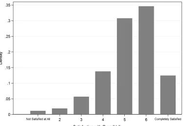
are you with your life overall?” This question is asked to all respondents every year in the
200
BHPS starting from 1996 (with the exclusion of 1997). Respondents have seven possible
categories among which to choose; these range from 1 to 7, where #1 is “not satisfied at
all”, #4 “not satisfied/dissatisfied”, #7 “completely satisfied”.
Figure 1 shows the distribution of life satisfaction across British individuals interviewed
between 1996 and 2008. The unconditional mean for life satisfaction reported over these
205
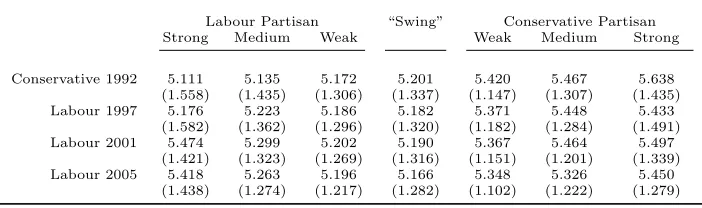
years is 5.2, with a median of 5. Table 1 shows the mean of life satisfaction during the
different legislatures covered by the period 1996–2008, conditional on the respondents’
po-litical ideology (they have been classified according to their answers to the above-mentioned
questions on political partisanship).
These statistics lead to some preliminary observations: nonpartisan voters report, on
210
average, a lower life satisfaction than partisan voters (independent of their political
ori-entation), and Labour partisan voters report, on average, a lower life satisfaction than
Conservative partisan voters. Both observations suggest there could be reverse causality
of conducting the baseline analysis on the subsample of swing voters only.
215
As mentioned earlier, the literature on retrospective voting has recognized the
impor-tance of monetary and financial indicators in determining voting choices. Following Fiorina
(1978) and many others, we use a subjective indicator to account for these monetary and
financial factors, which we derive from the responses to the question“How is your financial
situation compared to last year?” Respondents can choose from three possible answers: the
220
financial situation isbetter, thesame as, orworse compared to last year. Taking these
an-swers, we construct the dichotomous variablesBetterF inandW orseF in, taking values of
one when respondents believe that their financial situation is, respectively, better or worse
than last year, and zero otherwise.
We also compute the respondents’ family-equivalized income in logarithmic term,5 and
225
we include this measure in all our estimations. Controlling for anobjectivemonetary measure
of the household income is fundamental because it allows us to interpret the subjective
assessment of the household financial condition (measured by BetterF inand W orseF in)
as a broader evaluation of the individual economic situation. Finally, we include a set of
controls that are usually employed in the literature of well-being and voting behavior: age
230
of respondents (linear and squared), sex and marital status. Summary statistics for these
controls are displayed in table 2.
3. The Models
The empirical strategy is based on testing the main assumptions of retrospective voting
models augmented by well-being measures to show that SWB explains voting intentions
235
in addition to the usually employed financial indicators. Therefore, our hypothesis is that
through well-being indicators it is possible to capture the share of utility related to factors
that are not measurable in monetary terms.
We proceed as follows: We first start by replicating the main estimations employed
in previous research, to investigate whether voting decisions depend on financial situation
240
indicators. In particular, we include in the following estimation family income to account
5We follow the standard procedure of computing the equivalized income by dividing the total income
for an objective measure of family finances and, following Fiorina (1978), we use subjective
questionnaire responses of voters’ financial situation.
Accordingly, we first estimate our traditional model (Model 1):
SupportIncit=β1BetterF init+β2W orseF init+β3yit+γXit+ηt+ai+εit, (1)
whereSupportIncitreport the voting intention described in the previous section;BetterF init
andW orseF init are two dummy variables taking values of 1 if the respondent has replied
245
that her financial situation is respectively better or worse than in the past, aiming to capture
variations in utility due to monetary/financial components; yit is the natural logarithm of
the yearly family income, andXit is a vector of individuals’ personal characteristics (age,
sex, marital status, region of residence), note ; ηt denotes year effects; ai is an individual
effect (either random or fixed); andεitis the error term. The coefficients of interests areβ1
250
andβ2. Trivially,β1andβ3are expected to be positive, and β2, negative.
Next, we replaceBetterF initandW orseF initwith our well-being measures to account
for the subjective non-financial component of individuals’ utility. So we estimate the
well-being model (Model 2):
SupportIncit=δW ellbeingit+β03yit+γ0Xit+ηt+ai+εit, (2)
whereW ellBeing is constructed from respondents’ answers on life satisfaction. The
coeffi-cient of interest is nowδ,which is expected to be positive. Finally, we combine equations (1)
and (2) to estimate afull model (Model 3) where both well-being and financial indicators
are included as regressors:
255
SupportIncit=δ0W ellbeingit+β10BetterF init+β02W orseF init+β300yit+γ00Xit+ηt+ai+εit. (3)
We start off by estimating equations (1), (2), and (3) as a linear probability model
(LPM) with fixed effects (FE), to control for the within-variation effect of life satisfaction
on voting behavior. However, sinceSupportIncitis a dichotomous variable, we also propose
an alternative specification where we estimate the conditional probability of supporting the
incumbent party. For completeness of exposure, we do this by employing both a random
effect (RE) Probit and a fixed effect Logit, despite preferring the former to the latter.6 To
allow for correlation in the RE Probit between the model’s covariates and the unobserved
heterogeneity, ai, we apply Chamberlain’s method (1980) and assume the latter follows a
normal distribution with linear expectation and constant variance. So we augment our model
with a series of individual specific observable characteristics. By adding these variables,
265
Chamberlain’s RE probit essentially estimates the effect of varying the model’s covariates
while holding these individual’s specific characteristics fixed. 7
3.1. Baseline results
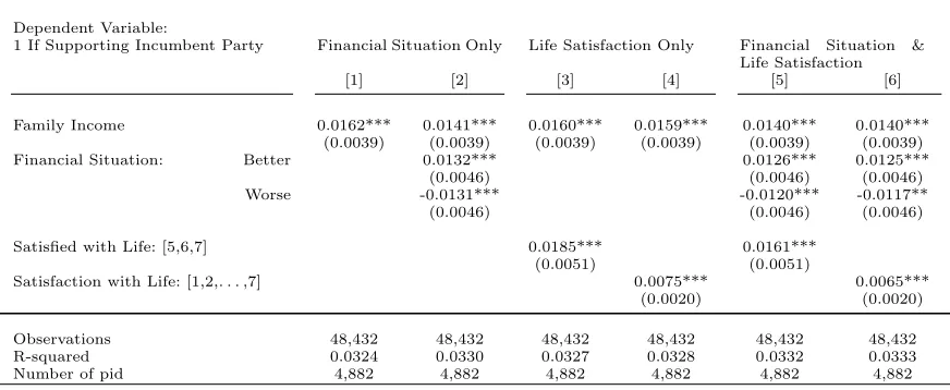
Results for the FE-LPM are displayed in table 3. Results for the RE Probit and for the
FE Logit are instead reported in the Online Appendix, in tables A.1 and A.2 respectively.8
270
There are 4,882 individuals who were interviewed for the entire period and for which we
have information on well-being and voting intentions. The dataset comprises nearly 50,000
observations.9 In columns [1] and [2] of table 3, we report the coefficients for Model (1),
the traditional retrospective voting model. Column [1] only controls for income, whereas
column [2] augments the model by also allowing for a subjective measure of wealth obtained
275
through the survey’s question on perceived changes in the household financial situation.
In columns [3] and [4], we display the results for Model (2), the well-being model. The
different columns use two variations ofW ellbeingit. First, we construct a dummy variable
taking the value 1 if the respondent has chosen the answer #5, #6, or #7 to the question
on life satisfaction and zero otherwise; this indicates that the respondent is satisfied with
280
life. Second, we treat the answers (from #1 to #7) to the question on life satisfaction as a
cardinal variable. Finally, in the last two columns, we propose the results of thefull model,
where both well-being measures and financial indicators are included, as in equation (3). All
6Given the short length of our dataset (we have a small time dimension of T=12), the incidental parameter
problem causes the FE Logit estimates of the parameters to be biased. In addition, we are interested in estimating the partial effect of our variables of interest.
7The vector of individual characteristics includes information such as whether the respondent regularly
reads newspapers, whether she ever smoked over the years, whether her partner has ever been out of employment, and what is the average income of her household.
8For the RE Probit, we display the average partial effect (APE) of the SWB variables at the bottom of
each regression.
9All results presented in the paper are based on this balanced sample. The baseline specifications
the regressions include the same controls, that is, marital status, sex, age, and age squared,
along with a set of region of residence dummies, and a set of wave-dummies. Standard
285
errors are clustered at the individual level.
Starting from the results on the traditional model, estimates from both the LPM (table
3) and the non-linear model (tables A.1 and A.2) are in line with the basic hypothesis
on the retrospective voting model, according to which one’s financial situation matters for
voting decisions. All the relevant coefficients are highly significant, at least at the 5%
290
level. In particular, respondents who believe that their financial situation has improved
compared to the previous year are more likely to support the incumbent compared to those
whose financial situation has not changed; the coefficients suggest that, approximately, the
effect is a 1.3% increase in the likelihood of supporting the incumbent. Respondents who
are instead worse off compared to the previous year appear to punish the incumbent by
295
reducing the likelihood of granting their support by approximately 1.3%. Finally, we note
that the income effect is quite small: an increase of 10% of the family income corresponds
to a small increase, approximately 0.14%, of the likelihood of supporting the incumbent.
Moving on to thewell-being model, where measures of subjective financial performances
are substituted with life satisfaction indicators, we can see that all the coefficients of interest
300
are again highly significant in all specifications, using both versions of well-being measures.
The magnitude of the response is similar to those recorded for the previous model: if a
respondent is satisfied with life, she will be about 1.8% more likely to support the incumbent
than if not. Similarly, using life satisfaction as a cardinal variable, an increase of 1 unit in the
life satisfaction scale is associated with an increase of about three quarters of a percentage
305
point in the likelihood of being pro-incumbent.10
In the final model, we include both indicators of well-being and of financial position.
We find that all indicators retain the same sign and magnitude as in the previous set of
regressions and they do not lose significance, which indicates that the two sets of measures
do capture different channels of support for the incumbent.
310
It is also interesting to compare the relative importance of subjective financial situation
measures with SWB ones. For the LPM displayed in Table 3 we compute y-standardised
10Remarkably, the coefficients related to the well-being variables for table 3, using an OLS estimator, are
coefficients as proposed by Winship and Mare (1984) and Long and Freese (2006) and we
can see that the probability of supporting the incumbent is 0.025 standard deviations higher
for those whose financial situation has improved, and 0.24 lower for those whose financial
315
situation has worsen off compared to those whose financial situation has not changed. For
SWB instead we see that an increase of 1 unit in the reported SWB (measured on a 1-7
scale) raises the probability of supporting the incumbent by 0.13 standard deviations.
In summary, our results support the idea that citizens’ well-being matters for voting
decisions, and in particular, our findings suggest that measuring utility in terms of only
320
monetary and financial indicators leaves out a component, which has a significant impact
on voting decisions.
3.2. Reverse causality? Tests on swing voters sample
In the voting literature, ideological preferences towards one party are generally assumed
to be exogenously distributed within the population. Some citizens are assumed to have
325
strong partisan preferences (either towards the incumbent or the challenger) while others are
assumed to be ideologically neutral. In this setting, voting decisions become the outcome
stemming from two different sources: the “ideological” component, originating from party
bias, and the “policy” component, resulting from actual governmental choices. The vote of
partisan citizens will be based on both the ideological and the policy related grounds, with
330
the weight of each component depending on the intensity of the individual-specific party
bias. The vote of ideologically neutral voters, instead, will swing exclusively in response to
government policies.
As we said above, partisan voters may experience higher levels of life satisfaction as
a consequence of their party electoral success or power endurance. This reverse causality
335
represents a bias for the estimation of our model; our strategy to reduce this bias is to classify
voters according to their political alignment and restrict the analysis to the voting behavior
of the ideologically more neutral group of swing voters. Since this type of respondents have
no (or very low)ex ante party preference, they should choose whom to vote mainly on the
basis of observed government’s policies.
340
Two questions asked in the BHPS allow us to split the sample between partisan voters
and ideologically neutral voters. The survey questions used to this purpose are (i)“Do you
answer“No”to both, we classify their position for that year to be one of a nonpartisan voter.
Almost 80% of individuals declared to be a nonpartisan at least once in the entire period.
345
Among this group, we define asswing voters those individuals who gave such answers more
than the half of median time during the whole survey, which is eight times or higher.11 This
subsample is constituted by 1,520 respondents, about 30% of the full sample. Using the raw
data, figure 2 shows that the share of respondents supporting the incumbent is higher among
individuals who declare themselves satisfied, and this difference is wider when one considers
350
only the swing voters sub-sample, which is consistent with the idea that ideologically neutral
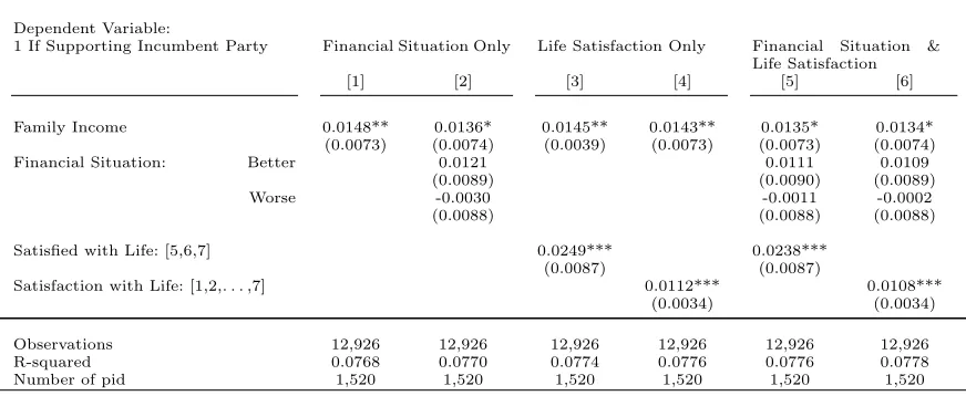
voters are more responsive to policies than partisan voters.
We employ this sub-sample to reestimate equations (1), (2), and (3). The results are
reported in Table 4, which has the same format as Table 3. The same set of controls are
used and standard errors are clustered at the individuals’ level.
355
The results confirm our hypothesis. First, the coefficients on well-being measures
re-ported in table 4 (and in tables A.3 and A.4 for the RE Probit and the FE Logit,
respec-tively) are still very significant and, generally, larger in magnitude than those presented in
tables 3. For example, looking at our preferred estimation, column [5] of table 4, the effect
forW ellbeingis now 0.0238 compared with 0.0161 in the corresponding column of table 3.12
360
Second, the positive effect ofimproved financial situation and the negative effect of worse
financial situation become non significant in all specifications. Third, the effect of family
income is still significant and similar in magnitude to the one in the full sample presented
in tables 3. Finally, note that in table A.6 of the online Appendix, as a robustness check,
we report the results for the estimation of Models (1), (2), and (3) for each level of life
365
satisfaction, for both the full sample and the restricted sample of swing voters. We observe
a pattern consistent with a positive relationship between the probability of supporting the
incumbent and the level of reported life satisfaction.
From the comparison of the coefficients on financial situation (better and worse) in
column [2] with the correspondent coefficients in columns [5] and [6] for the LPM in tables 3
370
and 4, we observe that the inclusion of SWB does not affect the estimation of the coefficients
11We have experimented with several other possible definitions of swing voters, depending on the number
of times the individuals answered the survey question regarding political ideology as described. These estimations bring similar results and are available upon request.
12Equivalently, looking at the y-standardised coefficients for the LPM in 3 and 5, in the full sample an
on financial indicators very much. This suggests that the correlation between well-being
measures and financial situation dummies is not high; so, in principle, both measures should
be included as covariates because they explain different components of voting behavior.
To expand on the results from the analysis of swing voters’ support to the incumbent
375
party, we need to address an additional concern regarding the possible endogeneity of
self-reported life satisfaction. As stated earlier, the wellbeing of partisan voters can be improved
by the mere fact that their preferred party holds power in the government or wins an election
campaign. Swing voters are not subject to this ideological bias, yet - when rational - they
are likely to experience an increase (decrease) in wellbeing, following the implementation of
380
beneficial (harmful) governmental policies. For this reason, the political science literature
argues that swing voters are often the target ofpersuasive campaigns, designed to resolve
their political independence and undefined party preference (see Mayer, 2008).
In the context of this paper, swing voters are defined on the basis of their dissociation to
any candidate political party. Two types of individuals fall into this definition: those who
385
have high interest in political matters, but are cynic and disillusioned by current politicians,
to the point of having no preference among available parties; and those who have low
interest in political matters, are not well informed about campaign programs and policies,
and therefore have no opinion about current politicians. Our conjecture is that the former
type of swing voters would highly reward (harshly punish) politicians who implemented
390
beneficial (harmful) policies, whereas the latter type of swing voter would experience low
wellbeing fluctuations in response to implemented policies.
We are not able to identify the source of variation in the wellbeing of swing voters, but
we can use personal characteristics and indicators of political involvement, in an attempt to
isolate those individuals who are likely to experience stronger reactions to the government
395
doing. In figure 3 we show that, as the number of waves an individual classifies as “swing
voter” augments, characteristics like average political interest, general election participation
rate, exposure to mainstream media and unions membership rate all decline. We exploit
these characteristics in table 5, where we replicate the estimation of Model (3) on two
separate samples of swing voters: those who define themselves as “fairly interested” or
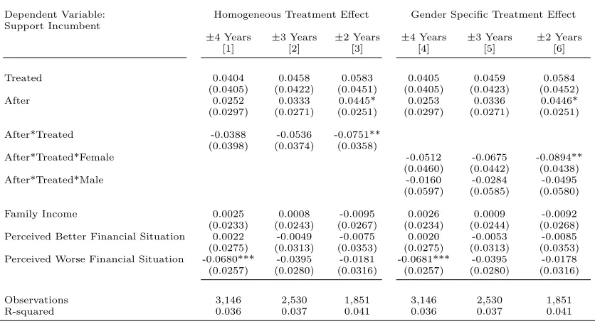
400
“very interested” in politics (columns [1] and [2]), and those who define themselves as “not
very interested” or “not at all interested” in politics (columns [3] and [4]). The results
case of swing voters with high political interest is double in size, with respect to the case of
swing voters with low political interest. This indicates that informed or politically-involved
405
voters who define themselves as non-partisan are the group that is most likely to increase
its support for the incumbent in response to changes in their level of life satisfaction. The
question remains on whether this difference is due to the fact that these swing voters are
those who are more sensitive to the consequences of implemented policies, and rationally
reward the incumbent party for the results achieved during their time in power.
410
As a final robustness check, we propose an alternative definition of swing voters, and test
the validity of our results. Always in figure 3, we show that there is a positive correlation
between the absence of strong party preferences, or political ideology, and the likelihood of
casting a vote in discordance with the pre-announced voting intention. To guarantee that
the definition of swing voters is based on elections that occur before the period during which
415
we observe our variable of interest, happiness, we focus on the two general elections of 1992
and 199713. This allows us to exclude the hypothesis that individuals fall into the “swing
voter” category because of low levels of wellbeing, due to contemporaneously implemented
policy. We select the sample of 1,305 respondents who declared to have participated in
these two early general elections, but qualify as “party switchers”: these are the respondents
420
whose actual vote went in favor of a party different from that mentioned as the one they
would have “most likely voted for in the coming elections”. Our definition of party switcher
differs from the one found in earlier literature, according to which the “floating voters” are
those switching supported party from one election to the others (see Zaller, 2004). Instead
of comparing actual votes across elections, we compare actual votes with vote intentions
425
reported in the time between elections. We believe this allows us to identify individuals
with high propensity of being persuaded by government actions, so we then replicate on this
sample the estimation of Model (3). As shown in columns [5] and [6] of table 5, the results
we obtain are strikingly similar to those from column [5] and [6] of table 4, both in terms
of coefficients significance and magnitude.
430
Overall we can say that, when taking out the ideological component from voting
inten-tions, using well-being measures generates even more consistent and significant results. We
investigate their relationship further in the next section.
13In this way we use characteristics that are predetermined with respect to the level of life satisfaction,
4. Exogenous Shocks of (Un)Happiness
In the previous section we have shown that using well-being indicators together with
435
financial indicators to proxy for utility is better than using only financial/economic measures.
We have established that when a voter reports a higher (lower) level of well-being, she is
also more (less) likely to support the incumbent.
In this section we present the results of an alternative exercise, which allows us to
address two points. First, it provides a further test to identify the effect of SWB on voting
440
intentions. Second, it allows us to test the hypothesis whether voters correctly attribute to
the government the responsibility of their well-being when they form their voting intentions.
Our identification strategy is: (i) to find an exogenous shock of happiness affecting only
some respondents, ourtreated group; (ii) to select a matched sample of individuals who did
not experience this shock (matched control group), but who have similarex ante probability
445
of experiencing the shock (propensity score matching); and (iii), to comparebefore-and
after-shock changes in political support responses of affected individuals to changes in political
support responses of unaffected individuals (DiD estimation).
Our priority is to exploit an exogenous shock that allows us to identify a connection
between a relevant event and the individuals personally affected by it. We exclude climate
450
changes and sports events, previously used in the literature, because we do not have data
on personal preferences about weather conditions or sport disciplines.14 We use, instead,
the death of the husband or wife as a shock of life satisfaction. This event, which is also
arguably beyond government’s control, is well known to have a deeptemporary impact on
well-being (see for example Clark and Oswald, 2002; Clark et al, 2008), and, its effect is
455
recognized to be stronger for women than men (Clark et al, 2002). Widowhood fits well
our purpose because it is possible to identify its exogenous component by using propensity
score matching.
14The UK Meteorological Office provides time series of climatic conditions, aggregated at the station-level
4.1. Propensity Score Matching
In order to be able to analyze the response to negative shocks of life satisfaction, such
460
as those caused by an event like widowhood, we need to deal with two problems. First,
a direct comparison between treated and untreated individuals is biased by the fact that
differences across these two groups depend on selection. Second, the time of the treatment
is respondent specific and cannot be imputed for the members of the non-treated group.
Propensity score matching provides a solution to both problems. It involves relying on a set
465
of observable characteristics that affect the “probability of being treated” (propensity score)
in an attempt to reproduce the treatment group among the non-treated. Imputation of the
time of treatment to the members of the control group is therefore made by pairing each of
its individuals with a member of the treated group. Becker and Hvide (2013) use a similar
approach to match firms with a deceased entrepreneur with firms where the organization
470
never experienced a similar shock, despite having similar characteristics to those who did. In
our setting, we use year of spouse death of treated respondents to impute the counterfactual
year of spouse death of the matched control. So, in this way, we are able to define before
and after spouse death for both treated respondents and matched controls.
We use nearest neighbor matching to select the group of individuals whose probability of
475
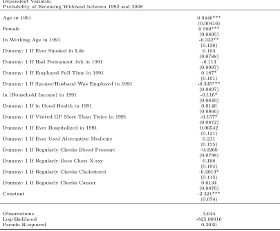
experiencing widowhood between 1992 and 2008 (the whole length of the BHPS), conditional
on characteristics observed in 1991, is the closest to that of the 363 individuals who did
experience widowhood over the same period.15 We begin computing the propensity score by
estimating a probit for the likelihood of becoming a widow. Table 6 provides evidence of the
good explanatory power of the chosen covariates, given the significance of their coefficients
480
and the highpseudo−R2of 0.30. We also estimated this model with a larger set of variables
controlling for a full set of personal, health-related, and financial characteristics. Other
explanatory variables not included in this preferred specification resulted as consistently
insignificant in all other robustness checks. The predicted probabilities estimated from this
model constitute our propensity scores. Before matching, the average propensity score is
485
0.352 for the treated group, and only 0.073 for the non-treated group. After imposing a
radius of 0.01 for the identification of the nearest neighbor to any individual belonging to
the control group, we discard 134 individuals and remain with a sample of 230 respondents
15This procedure involved omitting from the sample the individuals who had never been married, those
(153 of these are women and 77 men) who did experience widowhood and 230 matched
respondents who didn’t. In the matched sample, the average propensity score is reduced to
490
0.1963 for the treated group and 0.1952 for the control group. Histograms for the estimated
propensity score before and after matching and other more technical results are presented
in sections A.2 and A.3 of the Appendix.
4.1.1. DiD Setup
495
Our main focus is now to show that the spouse death negatively affects the probability
of supporting the incumbent, and that this negative effect fades away after three years from
the event; hence, it follows a pattern similar to the shock in SWB. We are mainly interested
in the differences after the event, but we also look into the behavior before the death to check
for the presence of any pre-treatment effect that could potentially invalidate our results.
500
Figures 4 and 5 provide graphical representations of how the drop in life satisfaction
translates into a reduction of support for the incumbent party. The figures display the
differences between thetreatedand theuntreatedindividuals during the year of the treatment
versus all other years. Thetreatment is defined as the respondent’s loss of a spouse, while
the years of widowhood refer to the year of the spouse’s death and to the following two
505
years. From the top left panel of figure 4, we can observe that treated individuals declare
themselves significantly less satisfied (withp−vlaue <0.01) during the years of widowhood
than during all other years, and from the top right panel we observe that, during the years of
widowhood, treated individuals are significantly less satisfied than the matched individuals
who did not experience the same shock (withp−vlaue <0.01). The bottom left and right
510
panels replicate the analysis on the expected incumbent support. Figure 5 presents the same
evidence in the form of an event study graph. In the top panel we observe clear similarities
between the probability of incumbent support and the probability of reporting high levels
of wellbeing for the treated group (solid lines), during the years preceding and following the
loss of a respondent’s spouse (normalized at period 0 for all respondents). As respondents
515
start experiencing lower levels of life satisfaction, between three and two years before the
loss of their spouse, we start seeing a decline in the support for the incumbent party. The
control group is not affected by the shock of the spouse loss, and both variables seem to
converge back to the same level around three years after the time of the shock. By looking
at the lower panels of figure 5, we notice that the group of treated females follows, for
both the incumbent support and the life satisfaction, a similar trend to the control group.
There is an increase in incumbent support two years before the spouse loss among female
treated respondents: this might cause concern regarding the presence of a pre-treatment
effect, which will be tested in the difference-in-difference analysis. Once again, this result
holds particularly for female respondents.
525
In order to analyze the dynamic of the probability of supporting the incumbent during
the years, controlling for potential confounding, assessing the magnitude and the statistical
significance of the effect represented in figures 4 and 5, we run a standard DiD regression,
where we compare treated and matched controls to assess how voting intentions are affected
by a spouse’s death (treatment). We estimate the following model:
530
SupportIncit=α+λ1×treatedi+λ2×af terit×treatedi+λ3×af terit+γ×Xit+δt+uit (4)
The coefficient of interest isλ2,which measures the difference between treated
respon-dents and control responrespon-dents after the treatment. The coefficient λ1 also presents some
interest because it constitutes a test for the lack of pretreatment effect. We include all
the controls that have been previously included in the regressions; these are age (in linear
and squared form), logarithm of family income, sex, as well as year and region dummies.
535
Standard errors are clustered at the individual level. We estimate equation (4) using the
Linear Probability Model.
Finding that the effect on the probability of supporting the incumbent in the treated
group lasts as long as the shock on life satisfaction and finding that the effect on women
is stronger than in men, would allow us to attribute the effect of the treatment on voting
540
intention to the shock of unhappiness.
4.1.2. DiD Main Results
We analyze whether individuals experiencing widowhood change their voting intention
differently than how do individuals whose spouses survive. Estimation results for equation
(4) and its variations are displayed in tables 7, 8, 9 and 10. In most of our regressions, we
545
consider windows over intervals of three and two years before and after the spouse death,
but we also experiment with shorter and longer periods.
to respectively 4, 3, and 2 years after and before the treatment. We observe that there is
a negative effect of widowhood on the probability of incumbent support; an effect which
550
is increasing and particularly significant in the sample restricted to the two-year window
(column [3]), suggesting that the widowhood-shock reduces by about 8% the probability
that the treated respondent gives support to the incumbent party. In table A.8, we obtain
more precise estimates of the effectduration, by estimating separate coefficients for the year
of the spouse death, the two years after, and simply the first and the second year after. The
555
effect of the shock on the incumbent support appears to be decreasing over time, consistently
with the pattern found on the life satisfaction variable.16 In these first three columns, we
impose the restriction that men and women react in the same way to the loss of their spouse.
However an analysis of the data, provided in the on line Appendix (Section A3), shows
that the effect of the spouse’s death on SWB is significantly higher for women than men.
560
This motivates us to analyze the responses by gender. We do it in two ways: (i) by
inter-acting af terit×treatedi with a dummy identifying the gender of the respondent; (ii) by
running separate regressions for male and female respondents. Columns [4] to [6] repeat the
estimates of columns [1] to [3], after relaxing the restriction of homogeneous treatment effect
across gender. We estimate different coefficients for men and women in the treated group.
565
Consistently with the asymmetry in the effect of this shock on life satisfaction, the results
show clearly that women are the ones whose voting behavior is affected by the spouse death;
theλ2are negative and become significant when we restrict the sample to two or three years
from the treatment. Again, we first start by estimating a commonλ2 for all years after the
spouse death. The results suggest that women are about 7% to 9% less likely to vote for the
570
incumbent following the death of their husband. When analyzing the duration of the effect,
we obtain significant and negative coefficients for women in the year of the event (about
-9%) and in the following year (about -12%) and a smaller nonsignificant effect two year
after the event (about -5%). Coefficients for men are smaller and nonsignificant. All in all
we can say that: the effect of the shock on the probability of supporting the incumbent party
575
follows the effect of the shock on the level of SWB.
As a robustness check, we run separate regressions for men and women. The results are
displayed in tables A.9 and A.10. From the inspection of the tables, we can clearly see that
16In the on line Appendix (Section A3) we provide a formal analysis on the impact of the spouse death
all the previous results are confirmed in terms of both magnitude and significance.17
4.2. Heterogeneous Responses: Income and Party Effect 580
There is a possibility that some of the individuals who experienced widowhood attribute
to the government partial responsibility for the loss of their spouse, maybe due to strong
existing dependence on national health programs, to changes in the succession law or to
unfavorable retirement policies. A possible objection is that, in all such cases, the loss of
one’s spouse corresponds to a sudden change in one’s personal financial condition, which
585
itself justifies increased support for a particular political party.
The results presented in section 4.1 do not support these arguments. We control for
wealth in all our estimations, measured as both objective income and subjective perceived
changes in own financial situation, and find it plays no significant role in explaining the
way individuals who experienced the loss of a spouse respond to voting intentions. Also,
590
we can argue that if the partner’s loss was perceived mainly in economic terms (i.e. as the
loss of a portion of the household’s income), then we would observe a permanent negative
effect. Instead, in the contest of this paper, we find only a temporary effect, suggesting that
widowhood affects voting behavior only for one, maximum two years after the shock.
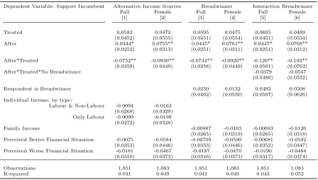
To elaborate further on our argument, we proceed by augmenting our
difference-in-595
difference setup with additional income controls. In table 8 we differentiate between
alter-native income sources (columns [1] and [2]), then we identify the respondents who qualified
as the household’s breadwinner for the majority of the years preceding the death of the
spouse (columns [3] and [4]), and finally we allow for the effect of widowhood to differ
ac-cording to weather the respondent was the breadwinner (columns [5] and [6]). If widowhood
600
was perceived as a sudden change in the household financial condition, then we should
ob-serve stronger effects on voting behavior of individuals whose spouse had consistently raised
the largest portion of the family income. Instead, we find that breadwinners, on average,
have the same expected voting intention of other respondents and that also their reaction
to widowhood is no significantly different from the reaction of other respondents.
605
17We can also observe that our matching technique has not left any pre-treatment effect, in Section 4.2
There is an alternative way to approach this issue. One can argue that a well-being
shock affects an individual social status and political bias (pro Labour Party, in this case),
rather than simply her support for the incumbent.18 A preliminary analysis suggests that
this argument does not hold in the empirical data. We only find evidence of a temporary
effect on incumbent support induced by the shock. We believe this hypothesis is instead
610
consistent with a long term (negative) effect of widowhood. To explore the issue further we
carry out additional robustness checks. The idea is that the effect of the shock on political
bias should take a different sign depending on the identity of the party in power, i.e. a
positive sign under left wing governments and a negative sign under right wing ones. We
can test this hypothesis of a widowhood-induced change in political bias directly, since the
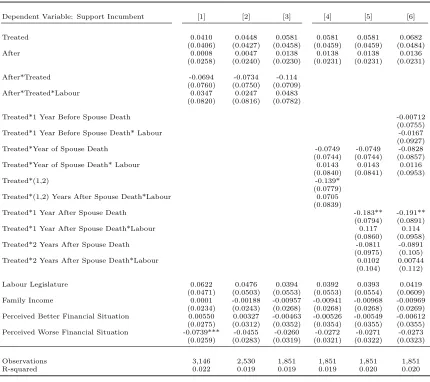
615
Conservative Party took over the Labour Party in 1996.19 We do this by re-estimating
equation (4) augmented with the interaction of the after treatment dummy with a temporal
dummy identifying whether or not the government in power is led by the Labour Party.
Table 9 presents our results. Columns [1] to [5] estimate the same models as the
corre-sponding columns of table 7 with the addition of the interaction terms. As we can see, the
620
results seem to confirm our hypothesis that there is no significant difference between the
two legislatures. The interaction of the after treatment dummy with the Labour temporal
dummy is always nonsignificant.20 Column [5] suggests that the probability of supporting
the incumbent in the first year following the spouse’s death is 0.183 lower for the control
than for the treatment group. This coefficient is comparable in magnitude and significance
625
with the effect found in column [5] of 7, our preferred specification (see also column [10] of
the same table). Column [6] tests the presence of pretreatment effect, and again finds that
voting behavior changes only after the spouse’s death.
4.3. Are voters rational?
We finally address whether individuals reward policymakers only for the increase in SWB
630
they are directly responsible for, or whether they also respond to events independent from
government actions. Assuming that experiencing widowhood in the U.K. during the period
1992-2008 is an event largely beyond government’s control, we convey that our preliminary
18Oswald and Powdthavee (2010, 2014) show that a shock that makes the individual more (less) needy
might increase (decrease) her support for a left wing party (i.e. the Labour Party in our case).
19Our dataset covers six years of Conservative Governments and eleven years of Labour Governments. 20The sign and magnitude of the coefficient would indicate that voting behaviour differs in legislatures
results seem to go in the same direction of a recent literature (Achen and Bartels (2004),
Healy, Malhotra, and Hyunjung Mo (2010) Wolfers (2002) Bagues and Esteve-Volart (2016))
635
showing how voters irrationally punish (or reward) policymakers for events that are
gov-ernment unrelated. We use the same strategy of section 4.2. to further expand on this last
point.
Blaming and punishing the government for the loss of one’s spouse would be classified
as rational behavior only if the responsibility of certain events could be traced back directly
640
to the government. This would be the case, for example, if the spouse had been victim
of negligence or malpractice on behalf of the NHS, for which the government in place is
ultimately accountable. However, if the government in place at the time of the survey
interview was different from the one in place at the time the shock was experienced by the
respondent, then a blaming attitude would still be classified as irrational.
645
We exploit the fact that in 1996 the Labour Party took power after two decades of
Conservative governments. Rational individuals whose spouse died during the Conservatives
years, should have stopped blaming their government once the Labour party came in power.
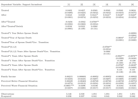
We construct an indicator variable Switchit, which equals one for the respondents whose
incumbent at the time of the interview is different from the incumbent at the time of the
650
spouse death.21 We then re-estimate an augmented version of equation (4) which includes
Switchitalong with its interactions to af terit×treatedi. Our conjecture is that if widows
wererationally blaming the government in power at the time of their spouse death, they
would have no reason to punish a government lead by a different party. A coefficient on
Switchit×af terit×treatedi significant and of opposite sign to the coefficient onaf terit×
655
treatedi would give evidence of such rational behavior.
Table 10 displays the results for this exercise. From the inspection of the table we
can clearly see that the newly introduced interaction is never significant. So we gather no
evidence that a switch of the party in power affects individuals response to the widowhood
shock, which would have indeed supported the conjecture of rational behavior.
660
5. Conclusion
Motivated by recent initiatives taken by governments and international organizations to
build measures of well-being that can be integrated with standard monetary and financial
measures to create informed policies, we test if well-being data can be used to predict voting
behavior.
665
Our aim is to contribute to the empirical literature on retrospective voting by augmenting
standard models of voting behavior with measures of well-being, to proxy for utility.
Pre-liminary results suggest that survey respondents modify their voting intentions in response
to changes in their level of life satisfaction.
The identification of the causal effect of SWB on voting intentions is the main source of
670
concern because of the potential for political ideology to enter the equation. For example,
a strong Conservative supporter may be satisfied by the simple fact that the Tories are
in power, rather than by the welfare enhancement brought by the party’s implemented
policies. We address this issue in two ways:(i) we split the sample between swing and
partisan voters, and we show that swing voters have a stronger reaction to a SWB shock
-675
the opposite behavior than would have taken place if our result were due to reverse causality;
and(ii) we use widowhood as an exogenous variation to identify the model - thus, allowing
us to conclude that changes in life satisfaction due to non-policy-related events also affect
respondents’ political intentions.
Having established that SWB measures are good indicators for predicting voters’
be-680
havior, we proceeded in the direction of asking whether or not voters are able to correctly
reward or punish the incumbent government only for the variation in life satisfaction that
can be directly attributed to government actions. People’s happiness depends on several
factors, and many of them cannot be directly linked to government action. To address this,
we test whether or not widowhood affects voters’ preferences toward incumbents. We use
685
DiD estimation and propensity score matching to identify the effect that widowhood has on
the probability of supporting the incumbent party. We find that a 1-point decrease in life
satisfaction measured on a 7-point scale corresponds to a 12% decline in the support of the
incumbent party. Consistent with our hypothesis, we find that the decline in support for
the incumbent party follows the same pattern as the decline in well-being that occurs in the
690
wake of widowhood. That is, the results follow the same trajectories. We confirm the above
a bivariate probit analysis.
Our analysis does not allow us to make predictions on electoral outcomes, as it does
not use actual voting data, and it exploits an exogenous shock that only affects a small
695
group of individuals. The paper allows us, instead, to evaluate the magnitude of the effect
of changes of SWB on voting behavior. The use of individual data and the identification
of a personal link between the exogenous shock and the affected respondents, we believe,
helps us understanding whether or not voters exhibit a rational behavior, which in turn
is important to predict policymakers decision and policy outcomes, as a recent important
700
paper by Asworth and Bueno de Mesquita (2014b) has shown. This paper makes a very
clear point that in order to understand policy outcomes it is important to understand how
voters form their voting choices, because elections are strategic interactions between relevant
actors (voters and policymakers).
We believe that our results have important implications. First, they motivate the efforts
705
taken by governments and international organizations in producing better and more
com-prehensive measures for well-being. Our results show that well-being plays a role in voters’
decision-making processes - a finding that is consistent with retrospective voting models,
and one that underscores the growing awareness of the importance of taking well-being into
account in policy formation. Second, they highlight citizens’ inability to correctly blame or
710
reward policymakers only for the actions they are responsible for. The results show that
voters fail to distinguish whether elected officials’ policies are responsible for a decline in
well-being they experience. Thus, a fall in a well-being - regardless of the cause - leads
voters to hold politicians in office responsible.
References
715
[1] Achen, C. H., Bartels, L. M., 2004. Blind retrospection: Electoral responses to drought,
flu, and shark attacks. Estudion Working paper 2004/199 https://www.ethz.ch/
content/dam/ethz/special-interest/gess/cis/international-relations-dam/
Teaching/pwgrundlagenopenaccess/Weitere/AchenBartels.pdf
[2] Ashworth, S., De Mesquita, E. B., 2014. Is voter competence good for voters?:
Infor-720
mation, rationality, and democratic performance. American Political Science Review,