Abstract—A new concept of discernibility degree of a condition attribute value and a new rough set theory based classification rule generation algorithm are proposed. The first key feature of the new algorithm, in comparison with standard rough set method and other rule induction methods, is its ability to calculate the core value without attributes reduction before; the second feature is not calculating the core values for the inconsistent examples; and the third feature is that in rule generation for inconsistent examples the condition attribute value that has the maximum discernibility degree should be selected first. Experimental results on 28 medical data sets show that the classification accuracy is much better than the standard rough set based classification algorithms, its variants, and a little better than C4.5, and RIPPERk.
Index Terms—C4.5, CBA, classification rule, rough sets, JRip
I. INTRODUCTION
ule learning has played an important role in machine learning and is known for inducing interpretable and comprehensible classifiers. Methods from statistical machine learning, on the other hand, have traditionally focused on predictive accuracy, often at the expense of interpretability. The goal of this work is to obtain highly predictive, yet interpretable classifiers.
The main rule based techniques are decision trees based rule learner [1], sequential covering [2], associative rules, and rough set [3] based methods, representative algorithms or softwares are C4.5, RIPPERk, CBA [4], and ROSETTA [5].
It is well known that C4.5 and RIPPERk are two excellent classifiers in classification performance, and there are little rule based algorithms comparable to them in classification accuracy[6-10] including the rough sets based classifiers.
Can rough set based rule generation methods be revised to get higher classification accuracy? This paper introduces a new rough set based rule generation method to construct a higher accuracy classifier compared to C4.5 and RIPPERk.
In standard rough set method an attribute reduction step
Manuscript received January 8, 2014; revised January 30, 2014 Honghai FENG is with the Institute of Data and Knowledge Engineering and School of Computer and Information Engineering of Henan University, Kaifeng, Henan, China. Phone: 86-371-23883088, email: [email protected].
Hongjing FENG is with Dalian Five Star Surveying and Mapping Techonology.
Yanyan CHEN is with Library of Henan University, Kaifeng, Henan, China..
Junhui Huang is with the Argumentum, No. 498 Guoshoujing Road Shanghai, .
should be carried out before rule generation, which may delete some important attributes and some attribute values may become indispensable that may not in original attribute set. And in standard rough set theory the method of inducing rules for the inconsistent examples are the same as for the consistent examples. However, the precision of the rules induced from inconsistent examples may be improved, because an inconsistent example in original decision table is a rule that has the original precision that may lower than the rule generated by selecting some of original condition attribute values as its antecedent.
In order to overcome these two shortcomings the new algorithm generates the core value for every consistent example first and generate rule on basis of it directly. And for inconsistent examples not generating core value first and selecting the condition attribute value first that has the maximum discernibility degree in rule inducing.
CBA use exhaustive search to find all the associative rules that satisfy the user-specified minimum support and minimum confidence. Two problems should be overcome in CBA that are the time complexity of exhaustive search and how to select good ones from very large amount of rules to final rules set to form the classifier.
RIPPERk producing decision lists are also known as sequential covering algorithms, since rules are learnt one at a time. For each rule, all instances covered by this rule are removed from the data set and the next rule is learnt from the remaining instances. The problem encountered in RIPPERk is that there are fewer rules induced to be selected for forming a better classifier.
C4.5 generates rules by transforming the decision tree into rules, the problem in C4.5 is that the post-pruning strategy, though its ability to avoid over-fitting in noise data sets, may reduce the accuracy in perfect data sets.
II. PRELIMINARY CONCEPTS OF ROUGH SET THEORY Rough set theory was developed by Zdzislaw Pawlak in the early 1980’s. It offers mathematical tools to discover patterns hidden in data. It can be used for feature selection, data reduction, decision rule generation, and pattern extraction etc.
A. Condition Attributes and Decision Attributes
Usually we distinguish in an information table two classes of attributes, called condition and decision (action) attributes. For example, attributes Headache, Muscle-pain and Temperature can be considered as condition attributes, whereas the attribute Flu as a decision attribute.
A Discernibility Degree and Rough Set Based
Classification Rule Generation Algorithm
(RGD)
Honghai FENG, Hongjiang FENG, Yanyan CHEN, and Junhui HUANG
B. Decision Systems/Tables
DS is a pair ( ,U A{ })d , U is a non-empty finite set of objects. A is a non-empty finite set of condition attributes such that :a UVa for every
a A
,V
a is called thevalue set of a.
d
A
, is the decision attribute (instead of one we can consider more decision attributes).C. Indiscernibility
The equivalence relation: A binary relationR X X , which is reflexive (xRx for any object x), symmetric (if xRy
then yRx), and transitive (if xRy and yRz then xRz). The equivalence class [ ]x Rof an element x X consists of all objects y X such that xRy. Let T = (U, A) be an information system, then with any BA there is an associated equivalence relation:
2
/ IS( ) {( , ') | , ( ) ( ')}
U IND B x x U a B a x a x
Where ( , ')x x IND BIS( ) is called the B-indiscernibility relation.
If ( , ')x x IND BIS( ), then objects x and x’ are indiscernible from each other by attributes from B.
D. Dispensable & indispensable attribute values for an example x
Suppose we are given a dependency CDwhere C is relative D-reduct of C. We say that value of attribute aC, is D-dispensable for xU, if
[
x
]
C
[
x
]
Dimplies[
x
]
C{a}
[
x
]
D (2)otherwise the value of attribute a is D-indispensable for x.
E. Attribute set independent for an example x
If for every attribute aC value of a is D-indispensable for x, then C will be called D-independent (orthogonal) for
x.
F. Value core for an example x
The set of all D-indispensable for x values of attributes in
C will be called the D-core of C for x (the value core), and will be denoted x( )
D
CORE C .
G. Value reduct for an example x
Subset C'C is a D-reduct of C for x (a value reduct), iff C'
is D-independent for x and
[x] C [x] Dimplies[x] C' [x] D (3) We have also the following property
( ) Re x( ) x
D D
CORE C
d C where Redx(C)
D is the family of all D-reducts of C for x.
H. Rough Membership
The rough membership function quantifies the degree of relative overlap between the set X and the equivalence class
[ ]
x
Bto which x belongs B: [0,1] X U .
| [ ] | ( )
| [ ] |
B B
X
B
x X
x
x
I.Decision Rule and its generalization
Each row of a decision table determines a decision rule, which specifies decisions (actions) that should be taken when conditions pointed out by condition attributes are satisfied. For example, the condition (Headache=no) and (Muscle-pain=yes) and (Temperature=high) determines uniquely the decision (Flu=yes). Objects in a decision table are used as labels of decision rules.
Given condition attributes set C
C C1, 2, ,Cn
and decision attribute set D, an example is an original and specific rule r in the form of (Ci C xi( )), CiC , with the rule strength
, if there is another attribute set R,RC exists; the rule
r
'of the form (CiC xi( )), CiR, with the same rule strength
, holds, and there are not any attribute set R'R, the other ruler
''of the form of(Ci C xi( ))
, '
i
CR, with the same rule strength
, holds, we have that R is one of the minimum reducts of example x with respect to C; andr
' is one of the generalization of the rule r of x.J.Inconsistent Decision Rule and Inconsistent Examples
Decision rules (or examples) that have the same conditions but different decisions are called inconsistent; otherwise the rules are referred to as consistent. Decision tables containing inconsistent decision rules are called inconsistent; otherwise the table is consistent.
K. Discernibility Degree of a Condition Attribute Value
Discernibility degree of a condition attribute value is defined as DIS that
( ( )) {j j( ) j( )}
DIS C x y C y C x
III. NEW CLASSIFICATION RULE INDUCTION ALGORITHM
A. Algorithm RGD
Input: Data set U, condition attribute set C, decision attribute set D
Output: Set of decision rules begin
getDIS(A, I);
getRules(); end
B. Method getDIS(A, I) begin
Attribute set A, instance set I
DIS A I( , ) for each example x
DIS A I( , ) { } x
for each attribute a
for each example y (
y
x
);if a x( )a y( )
add y to DIS A I( , )
endfor endfor endfor
return DIS A I( , )
end
C. Method getInconsistentExamples(instance inst)
begin
inconsistent example set INCON
for every example
x
iif ( ) ( ) i
D i A i
DIS x DIS x
add
x
ito INCONendfor return INCON
end
D. Method getCoreValue ()
begin
Core value set CORE
for every consistent example
if ( ) ( ( )- ( )) ( )
i j
D a a
DIS x DIS x DIS x INCON x ,
(i j)
add
a x
j( )
to COREendfor return CORE
end
E. Method getRules()
begin
rule set RULES
rule RULE
condition attribute set A
for every example x
if x is consistent
RULE (CiC xi( ))where C xi( )CORE x( )
for every condition attribute
C
j in A C iwhere( ) ( )
i
C x CORE x
add Cj C xj( ) to RULEthat maximize
( )
x
endfor endif
else if x is inconsistent
RULE(Ci C xi( )) that maximize
( )
x
for every condition attribute
C
j inA C
iadd Cj C xj( ) to RULEthat maximize
{ } { }
( )
i j
C C
x
endfor endelse endfor
add RULEto RULES
return RULES
end
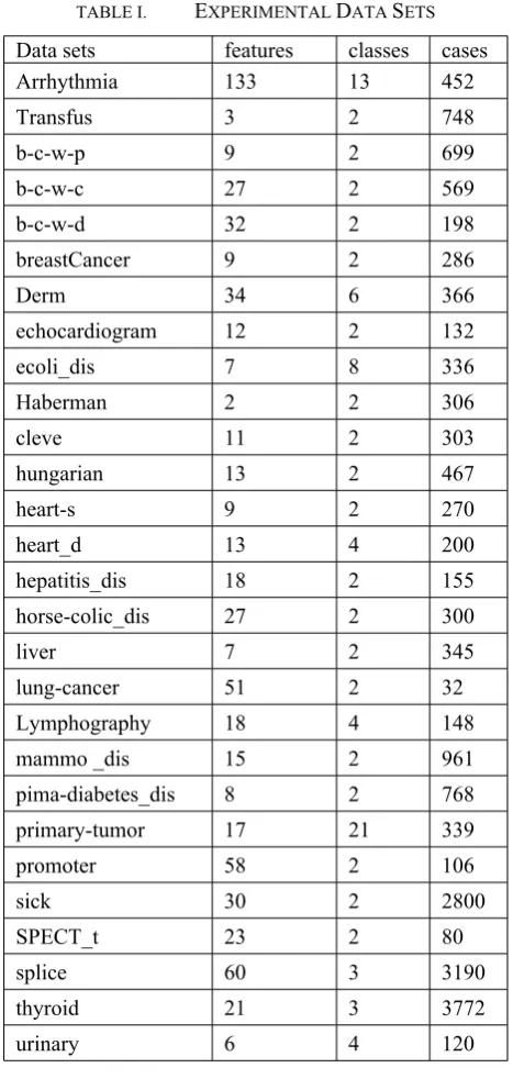
IV. EXPERIMENTAL DATA SETS
The data sets were obtained from the repository of Machine Learning databases at UCI [11], see their characteristics in Table 1. Some data sets are discretized by supervised discretization methods with WEKA and denoted as like australian_dis, and some data sets are discretized by unsupervised discretization methods with WEKA and denoted as like autos_undis. The original data sets and their corresponding abbreviation are as follows: Arrhythmia, blood_tranfusion(Transfus), breast-cancer-wisconsin (Prognostic)( b-c-w-p), sick_supdis(sick), primary-tumor, breast-cancer-wisconsin-cell-nucleus-diagnosis-superdis(b-c-w-c), mammographic_masses_supdis (mammo_dis),
breast-cancer-wisconsin-digitized-image-diagnosis-unsuperdis(b-c-w-d), breastCancer,
d), heart-c-supdis(heart-s), hepatitis_unsupdis(hepatitis_dis), horse-colic_supdis(hepatitis_dis), SPECT_train(SPECT_t), liver-disorders-unsupdis(liver), thyroid_supdis(thyroid), pima-diabetes_supdis(pima-diabetes_dis),
[image:4.595.52.286.124.616.2]promoter_gene(promoter).
TABLE I. EXPERIMENTAL DATA SETS
Data sets features classes cases
Arrhythmia 133 13 452
Transfus 3 2 748
b-c-w-p 9 2 699
b-c-w-c 27 2 569
b-c-w-d 32 2 198
breastCancer 9 2 286
Derm 34 6 366
echocardiogram 12 2 132
ecoli_dis 7 8 336
Haberman 2 2 306
cleve 11 2 303
hungarian 13 2 467
heart-s 9 2 270
heart_d 13 4 200
hepatitis_dis 18 2 155
horse-colic_dis 27 2 300
liver 7 2 345
lung-cancer 51 2 32
Lymphography 18 4 148
mammo _dis 15 2 961
pima-diabetes_dis 8 2 768
primary-tumor 17 21 339
promoter 58 2 106
sick 30 2 2800
SPECT_t 23 2 80
splice 60 3 3190
thyroid 21 3 3772
urinary 6 4 120
V. EXPERIMENT IMPLEMENTATION
With the Experimenter module of WEKA 14 rule based or tree based classification algorithms are compared with the new algorithm using a ten-fold cross validation procedure that performs 10 randomized train and test runs on the dataset. The 14 existing algorithms are CBA, ConjunctiveRule, DecisionTable, Explore, J48, JRip, LEM2, NNge, OneR, RandomTree, Ridor, Standard Rough Set, Variable Precision Rough Set, and ZeroR. Explore, LEM2,Standard Rough Set, and Variable Precision Rough Set are programmed with JAVA and embedded into WEKA 3.5.6. The others like JRip are from WEKA. The parameters in every algorithm are adopted default ones except that the minimum confidence in CBA is adopted 50%.
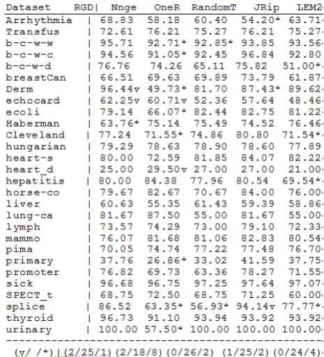
VI. EXPERIMENTAL RESULTS
Table 2 describes the experimental results in terms of percent correct. The first row lists the 15 algorithms, and the first column 28 data sets. The annotation v or * indicates that a specific result is statistically better (v) or worse (*) than the baseline scheme (in this case, the new algorithm RGD) at the significance level specified (currently 0.05). At the bottom of each column after the first column is a count (xx/ yy/ zz) of the number of times that the scheme was better than (xx), the same as (yy), or worse than (zz), the baseline scheme on the datasets used in the experiment.
Table 3 shows the comparison results about the 14 algorithms against RGD in term of 8 classification performance measures. The 8 measures are (1)mean absolute error, (2)percent correct, (3)weighted average area under ROC, (4)weighted average F-measure, (5)weighted average IR precision, (6)weighted average IR recall, (7)weighted average true negative rate, and (8)weighted average true positive rate. The other 6 measures (9-14) are for analysis of above performance measures, and they are (9) total length of all rules, (10) amount of attributes in the rule set, (11) mean length of the rules, (12) mean coverage of the rules, (13) mean accuracy of the rules. (14) amount of rules in the rule set.
VII. CONCLUSION AND DISCUSSION
(1) From the comparing results in Table 3 it shows that RGD achieve a good classification performance across the 28 medical data sets compared to other 14 algorithms.
(2) Among all the 15 algorithms NNge and Ridor are KNN variants and the others are rule or tree based methods. Among the rule or tree based methods CBA and RGD have the lowest measure of mean absolute error. The only consistent factor between CBA and RGD is that they all have higher rules’ mean accuracy. So we can infer that the measure of mean absolute error of a classifier is strongly related to the metric of mean accuracy of the rules.
(3)The rules in LEM2 have bigger mean coverage, but longer mean length and lower mean accuracy than RGD. The bigger mean coverage because LEM2 select the attribute values with biggest coverage to construct a rule. The longer mean length and lower mean accuracy is due to that LEM2 use the formula (1) as the stop schema when forming a rule, and as a result for an inconsistent example the rule's length is as long as the example itself, and the final classification performance is worsened.
(4) The two differences between RGD and Standard Rough Set are that Standard Rough Set has the attribute reduction step before rule generation and does not handle the inconsistent examples. So the metric of amount of attribute
in rule set in Standard Rough Set is very small (see Table 3) and may remove some significant attributes.
TABLE III. PERFORMANCE COMPARISON IN TERM OF 8 MEASURES OF
15 ALGORITHMS AGAINST RGD
(5) The measure of mean absolute error of J48 and Jrip is higher significantly than RGD, but in terms of percent of correct, weighted average IR recall, and weighted average true positive rate J48 ranks first. The significant feature of
CBA Conju Decis Explo J48 1. (2/21/5)(20/8/0) (18/10/0)(11/17/0)(8/19/1) 2. (2/25/2)(0/17/11)(0/17/11)(0/18/10)(1/27/0) 3. (2/23/3)(0/13/15)(1/15/12)(1/14/13)(1/26/1) 4. (3/24/1)(0/16/12)(1/16/11)(0/19/9) (4/23/1) 5. (3/23/2)(0/15/13)(1/13/14)(1/18/9) (4/23/1) 6. (2/25/1)(0/19/9) (1/17/10)(0/19/9) (6/22/0) 7. (3/23/2)(1/14/13)(2/14/12)(1/19/8) (4/23/1) 8. (2/25/1)(0/19/9) (1/17/10)(0/19/9) (6/22/0) 9. (0/0/28) (*/*/*) (*/*/*) (19/2/7) (*/*/*) 10.(0/18/10)(*/*/*) (*/*/*) (6/15/7) (*/*/*) 11.(9/5/14) (*/*/*) (*/*/*) (19/2/7) (*/*/*) 12.(28/0/0) (*/*/*) (*/*/*) (21/2/5) (*/*/*) 13.(10/6/12)(*/*/*) (*/*/*) (6/14/8) (*/*/*) 14.(0/0/28) (*/*/*) (*/*/*) (19/2/7) (*/*/*) Jrip LEM2 NNge OneR Rand 1. (10/17/1)(3/25/0)(0/24/4)(7/15/6) (2/26/0) 2. (1/27/0)(0/22/6) (1/25/2)(0/19/9) (1/23/4) 3. (1/23/4)(0/22/6) (0/20/8)(0/12/16)(0/24/4) 4. (1/27/0)(0/25/3) (2/26/0)(1/17/10)(0/26/2) 5. (1/27/0)(0/27/1) (1/26/1)(0/18/10)(0/25/3) 6. (1/27/0)(0/24/4) (2/25/1)(2/18/8) (0/26/2) 7. (3/22/3)(1/25/2) (2/25/1)(1/15/12)(1/22/5) 8. (1/27/0)(0/24/4) (2/25/1)(2/18/8) (0/26/2) 9. (*/*/*) (11/3/14) (*/*/*) (*/*/*) (*/*/*) 10.(*/*/*) (3/24/1) (*/*/*) (*/*/*) (*/*/*) 11.(*/*/*) (28/0/0) (*/*/*) (*/*/*) (*/*/*) 12.(*/*/*) (16/6/6) (*/*/*) (*/*/*) (*/*/*) 13.(*/*/*) (0/9/19) (*/*/*) (*/*/*) (*/*/*) 14.(*/*/*) (4/1/23) (*/*/*) (*/*/*) (*/*/*) Rido Stan VPRo Zero
1. (0/20/8)(11/17/0)(12/15/1)(23/5/0) 2. (1/27/0)(1/18/10)(2/16/10)(0/8/20) 3. (0/24/4)(0/19/9) (0/21/7) (0/6/22) 4. (3/25/0)(1/20/7) (1/18/9) (0/6/22) 5. (3/25/0)(1/19/8) (1/18/9) (0/3/25) 6. (2/26/0)(1/20/7) (2/18/8) (0/9/19) 7. (4/24/0)(0/20/8) (0/20/8) (0/4/24) 8. (2/26/0)(1/20/7) (2/18/8) (0/9/19) 9. (*/*/*) (16/9/3) (16/7/5) (*/*/*) 10.(*/*/*) (0/10/18)(0/10/18) (*/*/*) 11.(*/*/*) (26/2/0) (24/0/4) (*/*/*) 12.(*/*/*) (10/13/5)(16/10/2) (*/*/*) 13.(*/*/*) (7/17/4) (7/10/11) (*/*/*) 14.(*/*/*) (1/9/18) (2/9/17) (*/*/*)
1. Mean_absolute_error 2. Percent_correct 3.Weighted_avg_area_under_ROC
4. Weighted_avg_F_measure 5.Weighted_avg_IR_precision 6. Weighted_avg_IR_recall
7.Weighted_avg_true_negative_rate 8. Weighted_avg_true_positive_rate 9.Total_Length_of_All_Rules 10. amount of attributes in the rule set
11.mean length of the rules 12.mean coverage of the rules
[image:5.595.59.292.52.309.2]J48 and Jrip is their pruning technique that generates many rules with larger coverage but lower accuracy resulting the lower measure of mean absolute error and higher measure of percent of correct.
REFERENCES
[1] Ross Quinlan, “C4.5: Programs for Machine Learning,” MoRGDn Kaufmann Publishers, San Mateo, CA, 1993.
[2] William W. Cohen, “Fast Effective Rule Induction,” In: Twelfth International Conference on Machine Learning, 1995, pp. 115-123. [3] Z. Pawlak, “Rough sets,” International Journal of Computer and
Information Sciences, vol. 11, 1982, pp. 341-356.
[4] Bing Liu, Wynne Hsu, Yiming Ma, “Integrating Classification and Association Rule Mining,” In: Fourth International Conference on Knowledge Discovery and Data Mining, 1998, pp. 80-86.
[5] A Rough Set Toolkit for Analysis of Data,
http://www.lcb.uu.se/tools/rosetta/
[6] F.A. Thabtah, P.I. Cowling, “A greedy classification algorithm based on association rule,” Applied Soft Computing. vol. 7 , 2007, pp. 1102–1111.
[7] X. Yin, J. Han, “CPAR: classification based on predictive association rule,” in: Proceedings of the SDM, San Francisco, CA, 2003, pp.369– 376.
[8] TJEN-SIEN LIM , WEI-YIN LOH, “A Comparison of Prediction Accuracy, Complexity, and Training Time of Thirty-Three Old and New Classification Algorithms,” Machine Learning, vol. 40,2000, pp.203–228.
[9] Fadi Thabtah, Peter Cowling, and Suhel Hammoud, “Improving rule sorting, predictive accuracy and training time in associative classification,” Expert Systems with Applications, vol. 31, 2006, pp. 414–426.
[10] Renpu Li, Zheng-ou Wang, “Mining classification rules using rough sets and neural networks,” European Journal of Operational Research, vol. 157, 2004, pp. 439–448.