Abstract — This paper provides procedures for constructing prediction limits on order statistics of future samples using the results of a previous sample from the same underlying inverse Gaussian distribution. Prediction limits are obtained from a point of view of frequentist approach. Bayesian methods are not considered here. The results have direct application in reliability theory, where the time until the first failure in a group of several items in service provides a measure of assurance regarding the operation of the items. The prediction limits are required as specifications on future life for components, as warranty limits for the future performance of a specified number of systems with standby units, and in various other applications. Prediction limit is an important statistical tool in the area of quality control. The lower prediction limits are often used as warranty criteria by manufacturers. The technique used here does not require the construction of any tables. It requires a quantile of the Gθθθθ and F distributions and is conceptually simple and easy to use. The prediction limits obtained in the paper are generalizations of the usual prediction limits on observations or functions of observations of only one future sample. For illustration, a numerical example is given.
Index Terms — Future samples, order statistics, prediction limits
I. INTRODUCTION
HE inverse Gaussian distribution is a well-known distribution whose properties and applications have a remarkable similarity to those of the normal distribution (Chhikara and Folks [1], Folks and Chhikara [2]). It arises as the distribution of the first passage time of a Browning motion with positive drift and so it is logical to use it as a lifetime model. For example, as outlined in Chhikara and Folks [1], it has been used to describe the time for a reservoir to empty, to describe the interpurchase time for a consumable commodity, to model the time to failure of a device, or to model the distribution of strikes. Dennis, Munholland, and Scott [3] used it to describe the time to extinction of endangered species. For skewed data, the inverse Gaussian distribution has advantages over the Manuscript received March 23, 2014; revised April 10, 2014. This research was supported in part by Grant No. 09.1544 from the Latvian Council of Science and the National Institute of Mathematics and Informatics of Latvia.
Nicholas. A. Nechval is with the Statistics Department, EVF Research Institute, University of Latvia, Riga LV-1050, Latvia (e-mail: [email protected]).
Konstantin N. Nechval is with the Applied Mathematics Department, Transport and Telecommunication Instutute, Riga LV-1019, Latvia (e-mail: [email protected]).
Vadim Danovich is with the Cybernetics Department, University of Latvia, Riga LV-1050, Latvia (e-mail: [email protected]).
Gundars Berzins is with the Cybernetics Department, University of Latvia, Riga LV-1050, Latvia (e-mail: [email protected]).
traditional lognormal, gamma, or Weibull distributions in that a comprehensive methodology now exists similar to that of a normal distribution.
In this paper we discuss predictive inferences for the inverse Gaussian distribution, which was proposed by Chhikara and Folks [4], among others, as a lifetime model. The sampling theory and statistical methods for inverse Gaussian parametric estimation and hypothesis testing are well developed and are shown to have close analogy with their counterparts for the normal (Folks and Chhikara [2]). However, for certain applications in reliability and other fields (Banerjee and Bhattacharyya [5], Lancaster [6], Whitmore [7], and Folks and Chhikara [2]), it may be desirable to obtain confidence limits not for a parameter of the distribution, but for a future random observation drawn from the inverse Gaussian distribution itself. Such limits are called prediction limits. Statistical prediction limits have many applications in quality control and in reliability problems and the determination of these limits has been extensively investigated, particularly for the normal distribution. When the characteristic of interest is measured in time, say failure or repair time, distributions other than the normal are generally more appropriate. The gamma and Weibull distributions are frequently applied in studying the properties of life-time phenomena and there are several publications on the subject of their prediction intervals (see, for instance, Aitchison [8]).
Prediction limits can be of several forms. Hahn [9] dealt with simultaneous prediction limits on the standard deviations of all of the k future samples from a normal population. Hahn [10] considered the problem of obtaining simultaneous prediction limits on the means of all of k future samples from an exponential distribution. In addition, Hahn and Nelson [11] discussed such limits and their applications. Mann, Schafer, and Singpurwalla [12] gave an interval that contains, with probability γ, all m observations of a single future sample from the same population.
Fertig and Mann [13] constructed prediction intervals to contain at least m − k + 1 out of m future observations from a normal distribution with probability 1−β. They considered life-test data, and the performance variate of interest is the failure time of an item. Their lower prediction limit constitutes a “warranty period”.
This paper develops prediction limits (or one-sided prediction intervals) for future order statistics coming from the inverse Gaussian distribution, using classical frequentist approach. In the former case, the statistical prediction limits can be easily obtained when one parameter is assumed known and the other unknown, as well as when both are unknown.
Predictive Inferences for Future Order Statistics
Coming from an Inverse Gaussian Distribution
Nicholas A. Nechval, Member, IAENG, Konstantin N. Nechval, Vadim Danovich, Gundars Berzins
II. MATHEMATICAL PRELIMINARIES
A. Constructing Prediction Limits on Future Order Statistics under Certainty of Underlying Models
In this section, we consider the determination of prediction limits on future order statistics under certainty of underlying models. The following results hold.
Theorem 1. Let Y1≤ … ≤ Yl be the l ordered observations
in a sample of size l from a probability distribution (continuous or discrete) with density function gθ (y), distribution function Gθ (y), where θ is the parameter (in general, vector). Then a lower (1−α) prediction limit h on the kth order statistic Yk, k∈{1, …, l}, in a set of l future
ordered observations Y1 ≤ … ≤ Yl is given by
[
θ > = −α]
=argP{Y h} 1
h k
+ − + = =
− +
− α
θ
1 ; 2 ), 1 ( 2
) 1 ( ) ( arg
k k l
f k l k
k h
G , (1)
where f2(l−k+1),2k;1−α is the quantile of order 1−α for the F
distribution.
Proof. If there is a random sample of l ordered observations Y1≤…≤Yl from a known distribution
(continuous or discrete) with density function gθ (y), distribution function Gθ(y), then for the kth order statistic Yk
it is well-known that
j l j
l
k j
k G h G h
j l h
Y
P −
=
−
=
≤ }
∑
[ ( )] [1 ( )]{ θ θ
θ
) 1 , (
)
( − +
=IGθ h k l k
. )
1 ( )
1 , (
1 ( )
0
1 ) 1 ( 1
∫
− − − + −+ − Β =
h G
k l k
du u
u k
l k
θ
(2)
It follows from (2) that
∫
− + ++ −
− +
Β
− +
= ≤
) (
0
2 2 ) 1 ( 2 2 / ) 1 ( 2
2 ) 1 ( 2 , 2 2
2 ) 1 ( 2
} {
h
G l k k
k l
k u
k l k
l k l
h Y P
θ θ
− + − −
+ − − ×
− + −
2 1
2 / ) 1 ( 2
) 1 ( 2
2 )
1 ( 2
2 1
u du k
l k k
l k u
u l k
∫
∞
+ − −
− + − +
−
− +
Β
− +
=
) 1 ( 2
2 ) (
) ( 1
1 2
) 1 ( 2 2
/ ) 1 ( 2
2 2 , 2
) 1 ( 2
2 ) 1 ( 2
k l
k h G
h G
k l k
l
f k
k l l k l
θ θ
, )
2 ) 1 ( 2 1
( 2
2 ) 1 ( 2
df f
k k
l− + − l−k+ + k
+
× (3)
where
. ) 1 ( 2
2 1
+ − − =
k l
k u
u
f (4)
Thus,
+ − −
> =
≤ − +
) 1 ( 2
2 ) (
) ( 1 }
{ 2( 1),2
k l
k h
G h G F
P h Y
P k l k k
θ ϑ θ
θ
=1−
+ − −
≤
+ −
) 1 ( 2
2 ) (
) ( 1
2 ), 1 ( 2
k l
k h
G h G F
P l k k
θ θ
θ , (5)
where F2(l−k+1),2k has the F distribution with 2(l−k+1) and 2k
degrees of freedom. It follows from (5) that ]
1 } {
arg[ θ > = −α
= P Y h
h l =arg[Pθ{Yl ≤h}=α]
− =
+ − −
≤
= − + α
θ θ
θ 1
) 1 ( 2
2 ) (
) ( 1 arg 2( 1),2
k l
k h
G h G F
P l k k
=arg
(
Pθ{
F2(l−k+1),2k≤ f2(l−k+1),2k;1−α}
=1−α)
. (6)Since (from (6))
, )
1 ( 2
2 ) (
) ( 1
1 ; 2 ), 1 (
2 α
θ θ
− + −
= + − −
k k l
f k l
k h
G h G
(7)
we have that
α θ
− + − + − + =
1 ; 2 ), 1 ( 2
) 1 ( ) (
k k l
f k l k
k h
G . (8)
This ends the proof.
Corollary 1.1. Let Y1 ≤ … ≤ Yl be the l ordered
observations in a sample of size l from a known probability distribution (continuous or discrete) with density function gθ(y), distribution function Gθ (y). Then an upper α prediction limit h on the kth order statistic Yk, k∈{1, …, l},
in a set of l ordered observations Y1 ≤ … ≤ Yl is given by
[
θ > =α]
=[
θ ≤ = −α]
=argP{Y h} argP{Y h} 1
h k k
+ − + = =
+
− α
θ
; 2 ), 1 ( 2
) 1 ( ) ( arg
k k l
f k l k
k h
G
. /
) 1 ( ) ( arg
1 ); 1 ( 2 ,
2
+ − + = =
− +
− α
θ
k l k
f k l k
k h
G (9)
The main theorem, which shows how to construct lower (upper) simultaneous prediction limit for the order statistics in all of k future samples when prediction limit for a single future sample is available, is given below.
Theorem 2. Let mj “future” ordered observations
) ..., , ( 1
j j Ym
Gθ , where θ is the parameter (in general, vector), j∈{1, …, l}, and let ( , )
j
m k
Y denote the kth order statistic in the jth sample of size mj, where mj = m for all j∈{1, …, l}. Assume
that all of l samples from the same cdf Gθare independent. Then a lower simultaneous (1−α) prediction limit h on the kth order statistics ( , ),
j
m k
Y j=1, …, l, of all of l future samples is given by
− = > > >
=arg Pθ Y( , 1) h ,... ,Y( , ) h ,... ,Y( , ) h 1 α h l m k m k m k j = + − + + − = > = − + − − + − β α α θ 1 ; 2 ), 1 ( 2 1 ; 2 ), 1 ( 2 ) ,
( ( 1)
) 1 ( } { arg r r l r r l m
k r l r f
f r l h Y P + − + = = + − β θ ; 2 ), 1 ( 2 ) 1 ( ) ( arg k k m f k m k k h
G . (10)
Proof. If there are l independent samples from the same known distribution (continuous or discrete) with density function gθ (y), distribution function Gθ (y), then a lower simultaneous (1−α) prediction limit h on the kth order statistics ( , ),
j
m k
Y j=1, …, l, of all of l future samples may be obtained as follows:
> >
>h Y h Y h
Y P l m k m k m
k, 1) ( , j) ( , )
( ,..., ,..., θ
∏
= > = > = l j l m k j mk h P Y h
Y P
1 ( , ) ( , )
}] { [ θ θ
∑
= = − > > − − = l r j j l m k j mk h P Y h
Y P j l
1 ( , ) ( , )
}] { [ }] { 1 [
1 θ θ
) 1 , ( 1− 1 {(, ) } − +
= I−Pθ Yrm>h rl r
∫
> − − + − − − + − Β − = } { 1 0 1 ) 1 ( 1 ) , ( ) 1 ( ) 1 , ( 1 1 h Y P r l r m r du u u r l r θ∫
> − − + + + − − + Β − + − = } { 1 0 2 2 ) 1 ( 2 2 / ) 1 ( 2 ) , ( 2 ) 1 ( 2 , 2 2 2 ) 1 ( 2 1 h YP l r r
r l m r u r l r l r l θ − + − − + − − × − + − 2 1 2 / ) 1 ( 2 ) 1 ( 2 2 ) 1 ( 2 2 1 u du r l r r l r u
u l r
∫
∞ + − > − > − + − + − − + Β − + − = ) 1 ( 2 2 } { 1 } { 1 2 ) 1 ( 2 2 / ) 1 ( 2 ) , ( ) , ( 2 2 , 2 ) 1 ( 2 2 ) 1 ( 2 1 r l r h Y P h Y P r l r l m r m r f r r l l r l θ θ , ) 2 ) 1 ( 2 1 ( 2 2 ) 1 ( 2 df f r rl− + − l−r+ + r
+ × (11) where , ) 1 ( 2 2 1 + − − = r l r u u f (12)
r=1. (13)
Thus, > >
>h Y h Y h
Y P l m k m k m
k, 1) ( , j) ( , )
( ,..., ,..., θ + − > − > > − = −+ ) 1 ( 2 2 } { 1 } { 1 ) , ( ) , ( 2 ), 1 ( 2 r l r h Y P h Y P F P m k m k r r l θ θ θ = + − > − > ≤ + − ) 1 ( 2 2 } { 1 } { ) , ( ) , ( 2 ), 1 ( 2 r l r h Y P h Y P F P m k m k r r l θ θ
θ , (14)
where F2(l−r+1),2r has the F distribution with 2(l−r+1) and 2r
degrees of freedom. It follows from (14) that
− = + − > − > ≤
= −+ α
θ θ θ 1 ) 1 ( 2 2 } { 1 } { arg ) , ( ) , ( 2 ), 1 ( 2 r l r h Y P h Y P F P h m k m k r r l
=arg
(
Pθ{
F2(l−r+1),2r ≤ f2(l−r+1),2r;1−α}
=1−α)
. (15)Since (from (15))
, ) 1 ( 2 2 } { 1 } { 1 ; 2 ), 1 ( 2 ) , ( ) , ( α θ θ − + − = + − > − > r r l m k m k f r l r h Y P h Y P (16)
we have that
, ) 1 ( ) 1 ( } { 1 ; 2 ), 1 ( 2 1 ; 2 ), 1 ( 2 ) , ( β α α
θ + − + =
+ − = > − + − − + − r r l r r l m
k r l r f
f r l h Y
P (17)
where r=1. Taking into account (1) and (17), we obtain via Gθ(h) a lower simultaneous (1−α) prediction limit h on the kth order statistics ( , ),
j
m k
Y j=1, …, l, of all of l future samples as
[
θ > =β]
=argP{Y( , ) h}
h km
+ − + = = + − β θ ; 2 ), 1 ( 2 ) 1 ( ) ( arg k k m f k m k k h
G . (18)
This ends the proof.
Corollary 2.1. If k=1 and m1 = m2 = … = ml = m, then
− =
> > >
=arg θ ,... , ,... , 1 α
) , 1 ( ) , 1 ( ) 1 , 1
( h Y h Y h
+ = =
−α θ
1 ; 2 , 2
1 1 )
( arg
ml
mlf h
G . (19)
Proof.
> >
>h Y h Y h
Y P
l m m
m1) (1, j) (1, )
, 1
( ,..., ,...,
θ
∏
=
> =
> = l
j
l m j
m h P Y h
Y P
1
) , 1 ( )
, 1
( [ θ{ }]
θ
l
m h
Y
P{ }]
1
[ − (1, ) ≤
= θ
l
j m j
m
j
h G h
G j m
1
)] ( 1 [ )] ( [ 1
−
−
= −
=
∑
θ θ[
m]
l mlh G h
G ( )] [1 ( )]
1
[ − θ = − θ
=
j ml j
ml
j
h G h G j
ml −
=
−
−
=1
∑
[ ( )] [1 ( )]1
θ θ
∫
− −Β − =
) (
0
1 0
) 1 ( ) , 1 (
1 1
h G
ml
du u u ml
θ
−
> −
=
ml h G
h G F
P ml
2 2 ) (
) ( 1
1 2 ,2
θ θ θ
}, {
2 2 ) (
) ( 1
2 , 2 2 , 2 2
,
2ml P Fml f ml
ml h G
h G F
P = ≤
−
≤
= θ
θ θ
θ (20)
where
2 , 2
1 1 )
(
ml
mlf h
G
+ =
θ . (21)
This ends the proof.
Corollary 2.2. If there are l independent samples from the same known distribution (continuous or discrete) with density function gθ(y), distribution function Gθ(y), then an upper simultaneous α prediction limit h on the kth order statistics (, ),
j
m k
Y j=1, …, l, of all of l future samples with mj
=m is given by
=
> >
>
= Pθ Y h Y h Y h α
h
l m k m
k m
k, 1) ( , j) ( , )
( ,... , ,... ,
arg
= +
− +
+ − = > =
+ − + −
1 ; 2 ), 1 ( 2
; 2 ), 1 ( 2 )
,
( ( 1)
) 1 ( } {
arg β
α α θ
r r l
r r l m
k r l r f
f r l h Y P
. )
1 (
) ( arg
1 ; 2 ), 1 (
2
+ − + = =
+
− β
θ
k k m
f k m k
k h
G . (22)
III. THE INVERSE GAUSSIAN DISTRIBUTION
A random variable X is distributed as inverse Gaussian, denoted as X ~ IG(µ, λ), if its probability density function is given by
, 0 , 2
) ( exp 2
) (
2 2 2
/ 1 3
, >
−
−
= x
x x x
x g
µ µ λ π
λ λ
µ (23)
where parameters µ and λ are assumed to be positive; µ is the mean of the distribution and λ is a shape parameter. The probability distribution function is given by
− Φ
= 1
) (
, µ
λ λ
µ x x x
G
, 1 2
exp
+ − Φ
+
µ λ µ
λ x
x (24)
where Φ stands for the cumulative standard normal distribution function, and
− Φ
= −
=
µ λ λ
µ λ
µ x G x x x
G , ( ) 1 , ( ) 1
. 1 2
exp
+ − Φ
−
µ λ µ
λ x
x (25)
When both parameters µ and λ are known, the inverse Gaussian distribution function can be evaluated using the normal distribution table.
A. Estimation of Unknown Parameters
Let X1, X2, …, Xn be a random sample from (23). Tweedie
[14] showed that the maximum likelihood estimates (MLE’s) of µ and λ are
∑
= =
= n
i i
X n X
1
1
µ) (26)
and
∑
= −
−
= n
i Xi X
n 1
1 1 1 1
λ) . (27)
which are independently distributed with X~IG(µ,nλ) and nλ/λ~χn2−1,
)
where χv2 is a chi-squared random variable with v degrees of freedom. Furthermore (µ),nλ)−1) is a complete sufficient statistic for (µ, λ).
The MLE of the probability distribution function Gµ,λ(h) is now obtained by replacing µ and λ in (24) by their estimates µ)and λ)given in (26) and (27), respectively. Thus, the MLE of Gµ,λ(h) is
− Φ
= 1
) (
MLE
, µ
λ λ
µ )
)
h h h
G
exp 2 1 .
+ − Φ
+
µ λ
µλ )
)
) )
h
Accordingly, the MLE of Gµ,λ(h) is
− Φ
= −
=
µ λ λ
µ λ
µ )
)
h h h
G h
G ( ) 1 MLE, ( ) 1
MLE ,
. 1 2
exp
+ − Φ
−
µ λ
µλ )
)
)
)
h
h (29)
Chhikara and Folks [15] have given the minimum variance unbiased estimate (MVUE) of the inverse Gaussian distribution for different cases that might arise regarding µ and λ. When both of these parameters are unknown, it follows from their result that the MVUE of Gµ,λ(h) is given by
) (
MVUE , h
Gµλ
−
+ −
− +
> <
=
− −
− ( ) 2 1 4( 1) ( ),otherwise,
, 1
, 0
2 2 2 / ) 3 ( 1
2 T w
x nv
n n
n w T
U h
L h
n n
n
(30) and the MVUE of Gµ,λ(h) is given by
) (
MVUE , h
Gµλ
. otherwise ),
( )
1 ( 4 1 2 ) (
, 0
, 1
2 2 2 / ) 3 ( 1
2
−
−
+ − − −
> <
=
− −
− T w
x nv n n
n w T
U h
L h
n n
n
(31) where Tn−2 denotes the cdf of the Student's t distribution with (n−2) degrees of freedom and
, 1 1
1
∑
=
− = n
i xi x
v (32)
, ) ( ) (
) ( ) 2 (
2 1
x h n h h x n x v
x h n n w
− − −
− −
= (33)
, ) ( ) (
] / ) 2 ( [ ) 2 (
2 2
x h n h h x n x v
n h n x n n w
− − −
− + −
= (34)
, )
( 2
) ( ) 1 ( 4 ) 2
( 2
x v n
x nv x v n n x v n x L
+
+ − − +
= (35)
. )
( 2
) ( ) 1 ( 4 ) 2
( 2
x v n
x nv x v n n x v n x U
+
+ + − +
= (36)
IV. NUMERICAL EXAMPLE
An industrial firm has the policy to replace a certain device, used at several locations in its plant, at the end of 500-hour intervals. It doesn’t want too many of these items to fail before being replaced. Shipments of a lot of devices are made to each of three firms (l=3). Each firm selects a random sample of m=2 items and accepts his shipment if no failures occur before a specified lifetime has accumulated. The manufacturer wishes to take a random sample and to calculate the lower prediction limit so that all shipments will be accepted with a probability of 1−α = 0.95. The resulting lifetimes (in terms of 100 hours) of an initial sample of size n=46 from a population of such devices are given in Table 1.
TABLEI
THE RESULTING LIFETIMES (IN TERMS OF 100 HOURS ) Observations
Xi x1 x2 x3 x4 x5 x6 x7
Lifetime 0.2 0.3 0.5 0.5 0.5 0.5 0.6
x8 x9 x10 x11 x12 x13 x14 x15
0.6 0.7 0.7 0.7 0.8 0.8 1.0 1.0
x16 x17 x18 x19 x20 x21 x22 x23
1.0 1.0 1.1 1.3 1.5 1.5 1.5 1.5
x24 x25 x26 x27 x28 x29 x30 x31
2.0 2.0 2.2 2.5 2.7 3.0 3.0 3.3
x32 x33 x34 x35 x36 x37 x38 x39
3.3 4.0 4.0 4.5 4.7 5.0 5.4 5.4
x40 x41 x42 x43 x44 x45 x46
7.0 7.5 8.8 9.0 10.3 22.0 24.5
Goodness-of-fittesting. It is assumed that
−
−
=
i i
i i
x x x
x g
2 2 2
/ 1 3 ,
2 ) ( exp 2
) (
µ µ λ π
λ λ
µ
(xi ,µ,λ>0), i=1(1)46, (37) where the parameters µ and λ are unknown.
Considering the inverse Gaussian model for the data, unbiased estimates of µ and λ-1 are
, 61 . 3 1
1
= =
=
∑
=
n
i i
X n X
µ) (38)
1 1 0.60.
1 1
1
1 =
− −
=
∑
=
− n
i Xi X
n
λ) (39)
The maximum likelihood estimate of variance is given by
. 33 . 28 /
3 2=µ λ=
σ) ) ) (40)
inverse Gaussian and 0.0807 for the log normal, and these are smaller than their corresponding values expected at the five percent significance level. (The K-S test is considered in the sense that the unknown parameters of a distribution are estimated from the sample data.)
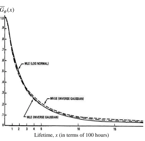
Now from (29) and (31) one is able to obtain the MLE and MVUE of Gθ(x), respectively. These estimates are given in Fig. 1 along with the MLE of Gθ(x)obtained from the log normal.
) (x Gθ
[image:6.595.49.291.174.409.2]Lifetime, x (in terms of 100 hours)
Fig. 1. Estimates of Reliability FunctionGθ(x).
Prediction limit. A lower (1−α) = 0.95 prediction limit h on the first order statistic Y1 in a set of ml = 6 future ordered observations Y1 ≤ … ≤ Yml is given by
] 1 } {
arg[ µ,λ (1, )> = −α
= P Y h
h ml
+ = =
−α λ
µ
1 ; 2 , 2 MLE
,
1 1 )
( arg
ml
mlf h
G
= × + =
= 0.0085
4 . 19 6 1
1 )
(
arg GµMLE,λ h = 0.22, (41)
where
− Φ
= 1
) (
MLE
, µ
λ λ
µ )
)
h h h
G
. 0085 . 0 . 1 2
exp =
+ − Φ
+
µ λ
µλ )
)
)
)
h
h (42)
Thus, the manufacturer has 95% assurance that no failures will occur in each shipment before h = 22 hours.
V. CONCLUSION AND FUTURE WORK
In this paper, we propose the technique of constructing prediction limits on future order statistics coming from the inverse Gaussian distribution under parametric uncertainty. These prediction limits are based on a previously available complete sample from the same distribution. We present an equation for this type of prediction limits which holds for any distribution and any statistic from the previous sample when a prediction limit for a single future sample is available. The prediction limits are found and illustrated with a numerical example. The methodology described here can be extended in several different directions to handle various problems that arise in practice. We have illustrated the proposed methodology for the inverse Gaussian distribution. Application to other distributions could follow directly.
ACKNOWLEDGMENT
This research was supported in part by Grant No. 06.1936, Grant No. 07.2036, Grant No. 09.1014, and Grant No. 09.1544 from the Latvian Council of Science and the National Institute of Mathematics and Informatics of Latvia.
REFERENCES
[1] R. S. Chhikara and L. S. Folks, The Inverse Gaussian Distribution.
Theory, Methodology and Application, New York: Marcel Dekker,
1989.
[2] J. L. Folks and R. S. Chhikara, "The inverse Gaussian distribution and its statistical applications - a review," Journal of the Royal
Statistical Society, Ser. B, vol. 40, pp. 263 –289, 1978.
[3] B. Dennis, P. L. Munholland, and M. J. Scott, "Estimation of growth and extinction parameters for endangered species," Ecological
Monographs, vol. 61, pp. 115 –143, 1991.
[4] R. S. Chhikara and L. S. Folks, "The inverse Gaussian distribution as a lifetime model," Technometrics, vol. 19, pp. 461– 468, 1977. [5] A. K. Banerjee and G. K. Bhattacharyya, (1976), "A purchase
incidence model with inverse Gaussian interpurchase times," Journal
of the American Statistical Association, vol. 71, pp. 823 – 829, 1976.
[6] A. Lancaster, "A stochastic model for the duration of a strike,"
Journal of the Royal Statistical Society, Ser. A, vol. 135, pp. 257–
271, 1972.
[7] G. A. Whitmore, "Management applications of the inverse Gaussian distributions," International Journal of Management Science, vol. 4, pp. 215 –223, 1976.
[8] J. Aitchison, "Bayesian tolerance region," Journal of the Royal
Statistical Society, Ser. B, vol. 26, pp. 161–175, 1964.
[9] G. J. Hahn, “Simultaneous prediction intervals to contain the standard deviations or ranges of future samples from a normal distribution," Journal of the American Statistical Association, vol. 67, pp. 938–942, 1972.
[10] G. J. Hahn, “A prediction interval on the means of future samples from an exponential distribution,” Technometrics, vol. 17, pp. 341– 345, 1975.
[11] G. J. Hahn and W. Nelson, “A survey of prediction intervals and their applications,” Journal of Quality Technology, vol. 5, pp. 178–188, 1973.
[12] N. R. Mann, R. E. Schafer, and J. D. Singpurwalla, Methods for
Statistical Analysis of Reliability and Life Data. New York: John
Wiley, 1974.
[13] K. W. Fertig and N. R. Mann, “One-sided prediction intervals for at least p out of m future observations from a normal population,”
Technometrics, vol. 19, pp. 167–177, 1977.
[14] M. C. K. Tweedie, "Statistical properties of inverse Gaussian distributions I," Annals of Mathematical Statistics, vol. 28, pp. 362– 377, 1957.