Automatic instance based matching of database schemas of web harvested product data

(1)

University of Twente

Automatic instance-based

matching of database schemas of

web-harvested product data

Author

Alexander

Drechsel

Supervisors

dr. ir. Maurice van

Keulen

dr. ir. Dolf

_Trieschnigg

dr. Doina

_Bucur

July 12, 2019

(2)

resam-pling the data with additional limiters . . . 42 4.1.7 Graphical Comparison between sampling methods . . . . 46 4.1.8 Comparison with the exact same datasets . . . 49 4.2 Experiments with using different machine learning algorithms . . 61 4.3 Experiments with prediction . . . 62 4.4 MacroScale Experiment . . . 72 4.5 Summary . . . 74

5 Conclusion 77

6 Future Work 80

(4)

Abstract

(5)

Chapter 1

Introduction

The general trend is that we register, record and do more and more things digi-tally. With evermore things happening on a digital level more of their underlying data sources which could contain valuable information are becoming available online. However they lack a standardized structure and individual data source structures can change from day to day. The content within these data sources is of course also continuously changing and expanding.

If one is able to consolidate the content of continuously changing data sources, which contain data they are interested in, into a single data source, and link all data which are about the same entity, in a cost efficient and thus preferably automatic way they could prove a very valuable source of operational or competitive advantage. In our research we will focus on data sources har-vested from websites but the developed system should be applicable to any data source containing data which is organized and linked together into items and properties. It should be applicable to all such data sources since in they are comparable in structure and preprocessing will take care of any difference in details that are caused by the format of its contents.

To consolidate different data sources, so they are in a single source and can be compared to each other, you need to determine both how the structures or schemas are similar to one another and once that has been determined, which data records refer to the same object. While studies[1, 2, 3, 4, 5, 6, 7] into auto-matically determining which records are the same across different data sources (also known as data fusion) as well as into computerized determination of data source schemas (what properties across data sources are identical in concept but are identified using different aliases) are not new research areas they both still remain open for ongoing research. Both topics are a challenge since they have to do with interpreting the meaning of table and attribute names and semantics remains a difficult topic for automation.

(6)

is often limited in those cases. For businesses as well as researchers for whom consolidating data is valuable it would be incredibly valuable to be able to more efficiently automatically consolidate information from big numbers of various data sources including ones with an unknown schema.

In both web harvesting and in the merging of data sources it often occurs that across different data sources data items such as products have properties which while identical in reality, use or concept are registered using different names. Since this concept is key to our research we will clarify that when we are talking aboutPropertieswe mean data of the same concept across all relevant data sources regardless of the actual name or alias used within those specific data sources. By this we mean data which may be grouped under a different name or alias is meant to mean the same thing in reality or in use. People have a ”first name” and a ”last name” but these can alternately be referred to as ”given name” and ”family name” or in different languages such as in dutch a ”first name” can be referred to as a ”voornaam” and a ”last name” can be referred to as ”achternaam”. These examples can be grouped into 2 properties, a ”first name” property which contains the data from ”first name”, ”given name”, and ”voornaam” and a property ”last name” which contains the data from ”last name”, ”family name”, and ”achternaam”. As an example from the test case of our research, which is about ball bearings and which was primarily gathered by harvesting data from webshops, each property of the bearings is described within each data source using a name or alias but the english name of ”inner diameter”, the dutch name of ”binnen diameter” and the domain specific abbreviation of ”d” all are referring to the same property. An experienced domain expert would quickly recognize this, but for a computer this would not be easy to learn.

(7)

(8)

Figure 1.2: A page from the website of the brand SKF of the 6017-2Z with various properties marked.

Presented above are two images of the same bearing from different websites. The two websites share many of the same properties but some properties are still differently named even though they mean the same thing. The product data gathered across websites may also be inconsistent such as in our example images the limiting speed being indicated differently between the websites. De-spite this similarities of data characteristics should be detectable for properties across websites. For example generally the product data harvested will contain a title and description describing each product and this will obviously be dif-ferent across products and websites. However when comparing the shape of the title and description properties they should possess similar shapes across the various data sources. Titles will generally be unique within a data source and each title will be of roughly similar length. These same data characteristics of uniqueness and length should also be similar for descriptions though the length of a description will likely be longer than that of titles.

(9)

should also be able to use a similar process to automatically determine which numerical properties across different data sources share the same meaning. In the case of numerical values such as various dimensions, weight and product identifiers we should be able to distinguish them from having distinct ranges and other characteristics.

There are a number of different methods by which data characteristics could be made comparable and thus to allow matching based on data similarity for properties. In our case we have chosen to use supervised machine learner based classification. We create our training data as well as process our test data by creating sets of characteristics which in the case of training data are labeled with the correct property. Our characteristics are based on calculations done over the aggregation of data values. Within each datasource we collect all data values that concern the same property. To ensure we have enough values to effectively use machine learning we do not calculate the characteristics based on all data values but instead split these data values up into a number of samples and calculate characteristics based on each of these samples.

Finding similarities to be able to link properties together on an aggregated level would be difficult for a human. Utilizing a machine learner however a computer should be able to handle most of the work and impartially detect similarities. By feeding aggregated characteristics about the data sources into a machine learner it should be able to develop a model capable of predicting to which already existing property new data would most probably belong to on the basis of its aggregated characteristics. Using this model and its predictions it should be possible to determine what properties are referring to the same concept.

Formally speaking the problem we are working on is one of schema matching. That is determining what property in one data source matches with a property in another data source and doing this for all properties involved to be able to determine a fully matching schema. To reduce the amount of work required to achieve fully matched schemas we want to develop a mostly automated method. Our approach to solving this problem is to utilize the similarity of data values of properties and determine schema matching on the basis of that.

1.1 Research Questions

1.1.1 Main Research Question

1. How can we link properties which represent the same real world property or concept together, using the characteristics and commonalities of their data.

1.1.2 Sub-Research Questions

(10)

2. How can a database or harvested web page be made suitable for linking properties together?

3. How can we best configure a machine learner and features representing data characteristics to perform content based property matching?

1.2 Validation and Approach

(11)

Chapter 2

Related Work

As the introduction discussed this research is about the linking of product prop-erties by the use of a machine learner and features built on data commonalities of the properties. In this section we will discuss the following:

• DIKW Pyramid: To explain the relation between data, information and knowledge.

• Machine Learning: As that is our primary method of solving our problem.

• Data Integration: To explain how our problem is placed in a greater whole.

• Record Linking: As the techniques used here can be made applicable to our problem

(12)

[image:12.612.134.478.143.423.2]

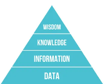
2.1 DIKW Pyramid

Figure 2.1: DIKW Pyramid

(13)

the similarities in their underlying data. In this context the structural informa-tion could also be considered data and by processing it with our methodology we can produce contextually useful information. In other terms we explore the data for commonalities and similar patterns to uncover hidden information. This hid-den information can then be used to structurally match data sources. By using the process and working with the data and information, we gain knowledge.

2.2 Machine Learning

Machine Learning is a broad field within computer science with many applica-tions pertaining to acquiring information from data and is capable of “learning” as the amount of suitable data increases. The concept of machine learning was postulated all the way back in 1950 by A.Turing [11] though the actual term was coined in 1959[12]. Since this research is an application of machine learning and there are multiple good books and papers available [13][14][15], this section will merely give a brief summary and how it is relevant for our research, referring interested readers to the referenced material and other information available.

There are multiple ways to categorise types of machine learning such as categorising based on its learning system and based on its desired output.

When categorising based on learning system or feedback signal there are two broad categories: Supervised Learning where the system is provided with a training set of example inputs and the goal is to learn of to match new data to the example data (in the form of the target outputs found therein). Within this category there are a few subcategories, Semi-Supervised Learning where the target outputs in the example data may be incomplete, Active Learning where the algorithm can query other data sources and the user for feedback during the learning in a limited manner and Reinforcement Learning wherein the training data is generated from a dynamic environment. The other category is Unsupervised Learning where the training data is not given any labels and he system is left to find structure and patterns on its own. Finding such patterns may even be the goal itself in such systems.

A different way of categorization is to base it on the desired output. In gen-eral machine learning tasks have similar desired output, which is the grouping or finding patterns in data. There are however a few distinct forms of output within this.

• Classification: Classifying inputs into distinct classes. Usually this is done using a learned model which has been built using labeled training data. Determining whether e-mail is in the class ”spam” or ”not spam” is an example of this.

• Regression: Similar to classification only the output is continuous, so in-stead of distinct separate classes it is assignment on a scale.

(14)

handling unlabeled data. Due to this it is often used to handle unsuper-vised learning tasks.

• Density Estimation: Used for estimated how a larger dataset may be distributed from a smaller sample.

• Dimensionality Reduction: A method to separate data into lower dimen-sionalities such as separating the contents of a library on the basis of topics.

The task we are working on for this thesis is the matching of database schemas. To accomplish this task we plan to match the different properties from databases on the basis of data commonality using supervised classifica-tion. After some preprocessing each database will have a number of feature sets created from each property. These feature sets represent the data in a machine learner processable format which can be used for the comparison and matching on the basis of data similarity. We also have manually created class labels for each property so that the correct match is known for the purposes of training. By taking these inputs we perform supervised classification with ma-chine learning. Our desired output is then the feature sets classified to belong to global properties. Combining this classification together with the link from which database level property each feature set was created from allows us to generate a database schema match for each used database to a global schema. The trained machine learner can then also be used to classify new databases to generate schema matches without the need to manually label the new database.

2.3 Data Integration

Data integration is the combination of different data sources about the same sub-jects to gain a consolidated and concise view of the data. Broadly speaking there are two methods by which data integration can be achieved.A<G,S,M>method such as described in [3] where the databases are not merged in actuality but has 3 elements allowing it to create unified views and process queries.

• A global database schema (G)

• Individual database schemas (S)

• Mappings (M) which define how to transform queries and results between the global database schema and each individual database schema.

(15)

1. Database schema matching and mapping, similar to the<G,S,M>method this is determining a global schema except the mapping is used to add all data from the individual databases into the global database instead of how to transform queries when they are called.

2. Duplicate Detection, determining which records refer to the same real world entities

3. Data fusion or data merging, merging the duplicates found together and dealing with the inconsistencies this generates.

This thesis focuses on providing an automated machine learning based method for the database schema matching step, primarily with the second methodology of actual database merging in mind but is applicable to the schema matching required for both methods of data integration.

2.4 Record Linking

While this thesis is interested in linking properties in an effort to provide au-tomation in schema matching, the techniques used in record linking for ”row-by-row matching are also relevant and applicable to our concept for data-driven schema matching. We make these techniques applicable by treating the prop-erties or columns of each data source as records. Thereby allowing us to match ”column-by-column”. The data contained in each column treated as the data which composes a record. Record linking is the task of linking records which refer to the same entity between multiple data sources. By linking records more complete information about entities can be built up. Record Linking can be considered a header for a field of linking methods and applications such as du-plicate detection (Often seen as part of a data integration process as described in 2.3), entity linking and entity resolution. There is a wide variety of meth-ods by which record linking can be done and the methmeth-ods are often used in conjunction. The following list explains a number of these methods.

• Standardization, as data can come from many different sources it is com-mon that data that contains the same information is often represented in different ways. Standardization or data preprocessing[16] works by ensur-ing all data which represents the same property is represented in the same way. Thus for example ensuring that dates are ordered in the same order and constantly use the same numerical or textual representation (2st of january 2019, 02/01/2019, 2 jan 2019, and 01/02/19 all being standard-ized to the same representation) or the same unit of measurement is used (lengths of 5 cm, 0,05 m, and 1.9685 in). Standardization can be achieved in a number of ways ranging from string replacement, tokenized replace-ment, or more complex methods such as hidden Markov Models[17].

(16)

threshold based on how many identifiers need to match. A similar method is also used internally by relational database which link their records to-gether using specifically defined primary keys.

• Probabilistic record linkage: while rule-based record linkage often looks for exact comparisons, by using probabilistic or fuzzy linking methods it is possible to roughly predict which records should be linked to each other. There is a variety of ways by which this fuzzy linking could be achieved[2] ranging from the simple addition of a edit distance to string comparison to the implementation of a Naive Bayes algorithm.

• Machine Learning, the general concepts of the above methods can also be enhanced and expanded by the application of machine learning techniques as well as opening other options.

2.5 Schema Matching

(17)

Figure 2.2: Tree Graphs from [6] which classifies schema matching approaches. The method proposed in this thesis is a instance based method using both linguistic and constraint approaches.

Regardless of how these approaches are categorized however it is important to note that what is explained in these sources are general approaches and not specific techniques on how to implement these approaches which can potentially be done via simple string comparisons or more complex methods such as using machine learning. Schema matching systems often combine these approaches in different ways using different implementations. As an example for how schema matching systems combine different approaches and implementations together: [5] describes a schema matching system called LSD which is used to integrate multiple data sources about real estate together. At its essence LSD uses 5 different techniques to match schemas together:

• Name Matcher which is a schema level linguistic matching approach im-plemented using a nearest neighbour based classifier called whirl[18] which has been developed specifically for text.

• Content Matcher which is a instance level linguistic matching approach based also implemented using whirl.

• Naive Bayes Learner is also an instance level linguistic matching approach except now implemented using a Naive Bayes learner where each instance is treated as a bag of tokens.

• County-Name Recognizer which uses auxiliary information to specifically recognise if a property is a county name.

(18)

When considering what schema matching approaches to use it is important to realize that different approaches requires different information which may not always be available.

• Constraints based approaches require that those constraints are known to the schema matcher.

• Using auxiliary information requires that such auxiliary information is available in a usable format.

• Matching based on usage requires that usage logs or some similar data is available.

• instance based approaches require that a sufficient number of instances is available to actually be able to use them to make determinations about the whole schema rather than just coincidental links.

(19)

Chapter 3

Approach

To merge separate data sources we need to find out how and where these sources fit together. This is a difficult task with multiple steps required. Our research attempts to provide a mostly automated method for the schema matching step of this process. We do this by using machine learning methods to match columns of tables or their equivalents based on the shape of their data.

Formally our task is to: Classify the properties of each data source such that those properties that are the same in concept are classified together. The classification should be based on the characteristics of the data of each property. To evaluate the success of our task we can exclude part of our data during the training phase of the classifier and evaluate the classifier using the accuracy scores of the predictions by the classifier for this excluded part of the data.

(20)

[image:20.612.134.478.152.378.2]

3.1 Processing Systems

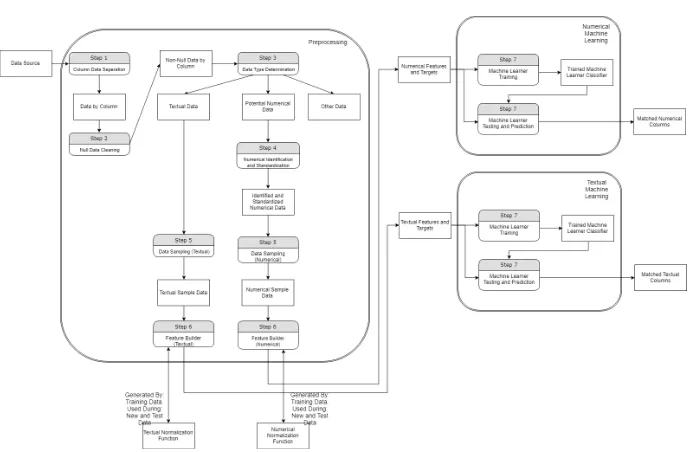
Figure 3.1: The flow diagram of the full design of the system and through what steps data go and are transformed into.

The process is divided into multiple steps: Pre-Processing Phase

Step 1. (Data Homogenization) Separate and transform the data sources into a homogeneous form. Since we are interested in specifically the properties of the data and want to determine how they are linked together based on similarity in shape we do not need to preserve all of the existing structure but instead only the core of what we are interested in. Since we are potentially dealing with multiple heterogeneous data sources of differing formats we can have multiple data transformation systems each of which designed to deal with a different data format. The end results for each of these systems will be the same: A series of headers each with a list of their associated data. We refer to such a data structure as a column.

Step 2. (Null Data Cleaning) Removal of all null and empty Data. This is im-portant since our test cases are using data harvested from the internet so we cannot expect 100% clean data and it is a given that this should be assumed to be the case for most real-life databases. Null and empty data are not relevant for our matching process and would only hinder our matching or cause errors.

(21)

of data for each property or column of data. Primarily this would split the properties into textual and numerical properties though other prop-erties such as dates and multiple propprop-erties concatenated together (such as Length x Width x Height) could be handled in a different manner and could be considered part of a different category than numerical and tex-tual, but we considered that outside our scope.

Step 4. (Numerical Identification and Standardization) Identification of the exact part of our numerical data that is actually the numeric value. This step contains 2 sub steps related to dealing with numerical values and their origin from different sources.

(a) Ensure that decimal and thousands markers are interpreted correctly. This is important since differing countries can use different characters to denote these markers.

(b) Identification and standardization of the units of measurements. This identification and standardization step is quite key since without it properties of the same type would not be fully comparable since char-acteristics such as ranges and averages would be calculated incor-rectly.

Step 5. (Data Sampling) To ensure we have the multiple data points needed for machine learning-based classification we divide our columns up into sam-ples of smaller size.

Step 6. (Feature Building) Calculation of sets of features from the samples of the now cleaned and standardized data. This step contains 2 substeps applying final data transformations related to the use of machine learning.

(a) Normalization of calculated features using the Unit Standard Devia-tion technique. We do this to reduce the effects of abnormalities and to ensure that all features are evaluated equally.

(b) Apply our manually created matches to the associated headers to add our desired target answers for later training and testing purposes.

Machine Learning Phase

(22)

[image:22.612.134.469.163.504.2]

3.2 Step 1. Data Homogenization

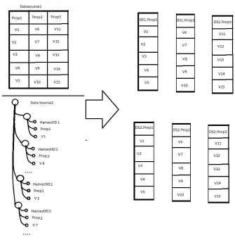
Figure 3.2: A visual representation of Data Homogenization.

In the Data Homogenization step we transform heterogeneous input into a ho-mogenous structured output to be used within the rest of the process. To do this we would have several systems which each handle one distinct type of input with the goal of each of these systems to generate the same output.

(23)

different data sources as well as to preserve potential hierarchies within the data source. Within the context of this paper we refer to this structure of a list of data values from a single data source headed by the property name they are associated with concatenated with its data source and hierarchy within that data source as a column.

Depending on the exact object type format of the data source, different systems are used. For relational databases the desired output is achieved by taking each table as an individual datasource and separating their columns into lists of data values, each headed by a column header which includes the full hierarchy of this column, meaning the data source, table name and column header concatenated together. Within our testcase of harvested ball bearing data from template-based websites such as webshops we have our data provided in the form of JSON files which have a structure as displayed in Figure 3.2 as Data Source2. For this type of data we load the JSON file as a list of lists and work downwards from the top adding each value to a new list of its matching property name, creating new lists when new property names are encountered. Similar systems would be created for any other format of data sources.

3.3 Step 2. Null Data Cleaning

Once all data has been translated into a universal format usable for our pre-processing steps we need to do some data cleansing. While later additional data cleaning may be required depending on what data type each part of the data set is determined to, be we can already do some cleaning at this point of unusable values. Specifically we can remove null and empty values, since those would only hinder the matching process or cause errors. Most of these values will be missing data rather than actual empty data that actually has meaning. To accomplish this, we simple run a checker over each column which removes unusable values.

3.4 Step 3. Data Type Determination

(24)

could include types such as datetimes where comparing should be done differ-ently due to the way days and months roll over and combined data types which include multiple values such as a dimensions property which includes height, width and length.

In theory distinguishing between textual and numerical data should be easy especially if we consider the textual data type to be default and we only really need to determine if data is numerical. However there are several factors which make it more difficult in practice. Firstly one of the intended purposes of this method and our research case is to enable the merging of web harvested data which mean that we need to be able to deal with dirty data or other forms of values where a numerical value may not purely consist of numerical characters. There are two levels where we need to consider when determining if we should consider data to be numerical. First we need to determine if a specific value is numerical and a column as a whole is numerical or otherwise.

On the level of columns we decided to use a percentage threshold which needs to be reached by individual values considered to be numerical. If this threshold is reached than all individual values that were not determined to be numerical will be discarded. We decided to discard these values since if the threshold is reached we are most likely dealing with a numerical based column in which case the non-numerical values would not be very useful since we are keeping the data types seperate and using those remaining values as textual data would result in small columns of data of insufficient size for productive matching.

When determining individual values it is important to consider a numerical value does not consist purely of numerical characters but that in the end we would prefer to only end up with numerical values. This means that we need to make allowances for values containing units of measurement, dots, commas, odd formats such as fractions and other additional text. At the same time how-ever there will be instances where we do not want to consider something to be numerical simple because it contains numeric characters. An example of such an instance would be alphanumeric codes (such as item codes) and compound values. While there are multiple approaches possible to solve these issues. The approach used in this research is a specialized regex or regular expression. Using the regex we account for the various difficulties but the regex expressions have been hand-crafted on the specific dataset and a better more generic solution should be possible. A good example of this specialized nature is the inclusion of see diagram image as that present due to some data sources containing nu-merical values where this section of text is present.

The regex expression we used for the data type determination is as follows: “[0-9]+[.]?[0-9]*[\- ]*([0-9]+/[0-9]+—/[0-9]+)?[\- ]*(rpm|mm|inch|in|degrees c.

|degrees f.||each|g|n|kn|lbf|kgf|lb|lbs)?[ ]*(see diagram image)?” The regex expression is dividablable into a number of sections.

• [0-9]+[.]?[0-9]*[\- ]*([0-9]+/[0-9]+|/[0-9]+) identifies the actual number

(25)

• (rpm|mm|inch|in|degrees c.|degrees f.||each|g|n|kn|lbf|kgf|lb|lbs)? is an enu-meration of units of measurement

• [ ]* spacing characters

• (see diagram image)? Section of text which occurs within some data sources contained within some of their numerical values

This regex expression is meant to identify numerical data within our dataset by full matching their data value. This also includes any text within the same data value. Units of measurement included in these data values are useful for identification and standardization performed in step 4. see diagram image is not useful in step 4 but is used in the matching process for completeness since it is present within the data and its inclusion allows us to use full matching instead of partial matching. Reducing the chance of incorrectly recognising a textual value as a numerical one because it happens to include a number. Due use of this regex it is likely that when new data sources are added this regex will need to be extended due to new units of measurements or other text included in numerically typed data.

3.5 Step 4. Numerical Identification and

Stan-dardization (Numerical Data only)

While extracting features beyond the shape of the data is difficult for textual data due to the difficulty in processing natural language this should not be the case for numerical data. If we want to extract additional features from numerical data however we do need to determine the actual number contained in each numerical value. To achieve this we need to take a number of steps. According to current standards[19] both dots and commas can function as the decimal separator and no thousands marker should be used this may not necessarily be the case for the data we are working with. The programing language we used considers a dot to be a decimal marker with commas having a different use. Thus we need to remove any possible thousands markers and ensure all comma decimal separators are replaced by dots.

Once we have accounted for the use of decimal and thousands separators we should now determine what part of the data values we are checking is the actual numeric value. Within our datasets we encountered three ways the actual numeric values were displayed.

• A number potentially with a decimal separator. – 70.5 is an example of this

• A number displayed as a fraction. – 2/3 is an example of this

(26)

– 2 1/3 is an example of this

To identify the actual numerical value in each of these cases we once again use regular expressions.

• Our data values still need to satisfy the regex used in the type deter-mination process so it should still satisfy “[0-9]+[.]?[0-9]*[\- ]*([0-9]+/[0-9]+—/[0-9]+)?[\- ]*(rpm|mm|inch|in|degrees c.|degrees f.||each|g|n|kn|lbf

|kgf|lb|lbs)?[ ]*(see diagram image)?”

• We check to see how many matches with ’[0-9]+[.]?[0-9]*’ we have. – If we have a single match this means we are dealing with the first

case and can simply change the string value to numerical value.

– If we have two matches and ’[0-9]+[.]?[0-9]*[\- ]*\/[\- ]*[0-9]+[.]?[0-9]*’ can be matched we are dealing with the second case. To acquire our actual numerical value we use division with our two matches to acquire our a decimal representation of our fractional

– If we have three matches and ’[0-9]+[.]?[0-9]*[\- ]*[0-9]+\/[0-9]+’ can be matched we are dealing with our third case. To acquire our actual numerical value we use add our first match to the division with the second and third matches to acquire our a decimal representation of our fractional

Once we have identified the actual numeric value we could consider this step a success but to aid in comparison we would also like to ensure that values of the same physical quality (Lengths, Weights and Force to give some examples) are all using the same unit of measurement. For our test case we simply have a se-quence of if/else statements checking for the presence of units of measurements and standardizing them towards the most common unit of measurement in their category. We standardize towards the most common unit of measurement in-stead of the SI standard since not all numerical values have units of measurement associated with them so converting to the most common should give the best results for comparison. The methods we are using here are somewhat simplistic and more complicated but better performing methods are possible.

3.6 Step 5. Data Sampling

To be able to properly use our data in machine learning for the purposes of classification we need to turn our data values into features of those values . However we need a sufficient number of such feature data for machine learning and not merely a single set of features per property. To have a sufficient number of feature data per property which each still is sufficiently characteristic enough about the property we propose to split the data we have up into samples.

(27)

[image:27.612.159.461.172.416.2]

be created. In the experiment section we will evaluate which of these methods performs best.

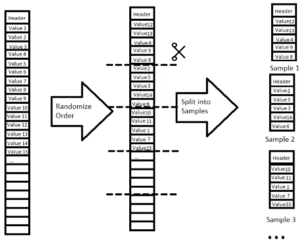
Figure 3.3: Data Split

(28)

Figure 3.4: Resamping

Figure 3.5: Resamping

(29)

within the same sample the same exact value entry cannot occur twice. In In-dividual Resampling a value never becomes unselectable, meaning that while extremely unlikely it is possible for a sample to be created from a single value entry repeated.

Figure 3.6: Resamping with Limiters

A final refinement added into the resampling creation process is the addition of limiters, clearly defining a minimum size a column needs to use it for the sampling process. and maximum limit in how many samples may be created from a column based on the proportional difference between the size of the column and the size of a sample. We called this method Resampling with Limiters.

We evaluate the performance of each of these sampling methods in section 4.1.

Since the goal is matching columns together, each created sample also has its original column and data source name associated with it so that it is traceable.

3.7 Step 6 Feature Building

With the various columns divided into samples the Feature Building step turns those samples into a format understandable to machine learners. By calculating various features for each sample we get numerical representations of the shape of the columns. The created features differ between the various data types since both what we have to work with and how they differ within their data type is different.

(30)

• The value of the most common entry within the sample

• The number of unique entries represented as a percentage to avoid the sample size from influencing this.

• The minimum numerical value within the sample

• The maximum numerical value within the sample

• The mean of all numerical values within the sample

• Standard Deviation within the sample

In the case of textual data part of the problem is that the machine learning algorithms that we use cannot utilize text directly, there are multiple ways to deal with this problem such as a representing it in numbers using a bag of words or other methods. For our purposes however we are trying to match based on the shape of the data and are trying to sidestep language issues because of this we instead calculate most features based on the character and word length of the data. For textual features we generate the following:

• The number of unique entries represented as a percentage to avoid the sample size from influencing this.

• The minimum amount of characters in a value within the sample

• The maximum amount of characters in a value within the sample

• The mean amount of characters within the sample

• Standard Deviation within the sample in terms of amount of characters

• The minimum amount of words in a value within the sample

• The maximum amount of words in a value within the sample

• The mean amount of words within the sample

• Standard Deviation within the sample in terms of amount of words Once the features have been built we have two transformation steps to perform as well.

(31)

of attribute the number transformed to will be the same. For example we have the column called Inner Diameter (d) from the data source xbearings referring to our manual match file this is associated with the attribute Inside Diameter and referred to by the number 4. The numbers used to refer to attributes are generated based on line the attribute is listed in the manual match file.

Secondly, we perform normalization on the generated features. We perform Unit Standard Deviation Normalization which means we express each feature in the form of the number of standard deviations it is away from the average of that feature across all features of its type. For example consider an inner diameter attribute which has a mean of 30, and a standard deviation of 5. By applying Unit Standard Deviation Normalization we express values into num-ber of standard deviations away from the mean instead. In our example this means that a value of 20 is normalized into -2 and a value of 35 into 1. This normalization is applied to each attribute meaning that all features are values roughly around 0. We do this normalization to aid in machine learning algo-rithms evaluating each feature equally. The functions used to apply this unit standard deviation normalization is also delivered as an output since the same normalization function needs to be applied to all data within the same machine learner. In the case of new data or data kept separate for testing purposes this normalization function produced as output is used instead of calculating one for just the new data.

3.8 Step 7. Machine Learner

With all the pre-processing steps finished we now have data in a machine learner ready format. Having the feature sets with their target answers in hand, the actual machine learning is fairly straightforward. The problem we are aiming to solve is the matching of similar columns. This is a classification task with each target being an attribute to which samples are associated to. We have a number of possible machine learning algorithms we can use for this task. Each of these algorithms also have some associated hyperparameters with a number of possible values. To determine the most optimal hyperparameter values we use grid search to exhaustively search for the best results within the training set.

Our possible machine learning algorithms with their associated hyperparam-eters are:

(32)

• LogisticRegression with a C of 10-3 through 103, increasing in steps of 1 exponent. This algorithm works by a series of boolean tests based on values of features to divide the dataset between the attributes.

• LinearSVC with a C of 10-3 through 103, increasing in steps of 1 exponent. This algorithm is a support vector classification (SVC) based algorithm, which means that attempts to divide the feature space between the differ-ent attributes by the use of function based lines. LinearSVC uses linear functions to define these lines.

• PolynominalSVC with a C of 10-3 through 103, increasing in steps of 1 exponent and a degree of 3.This algorithm is a support vector classifica-tion based algorithm, which means that attempts to divide the feature space between the different attributes by the use of function based lines. PolynominalSVC uses polynominal functions to define these lines.

• RbfSVC with a C of 10-3 through 103, increasing in steps of 1 exponent. This algorithm is a support vector classification based algorithm, which means that attempts to divide the feature space between the different attributes by the use of function based lines. RbfSVC uses radial basis functions (Rbf) to define these lines.

• SigmoidSVC with a C of 10-3 through 103, increasing in steps of 1 ex-ponent.This algorithm is a support vector classification based algorithm, which means that attempts to divide the feature space between the dif-ferent attributes by the use of function based lines. SigmoidSVC uses sigmoid functions to define these lines.

• Multinomial Naive Bayes which is a Naive Bayes based classifier suitable for multiple features.

3.9 Summary

By following the steps described in this chapter we can take data from different data sources and make them matchable on a data similarity level by use of a classification based machine learner and data characteristic based feature sets which have been calculated from aggregated samples.

The steps can be summarized as such:

1. Translate the data sources into a single homogenous format.

2. Clean the data from garbage data

3. Determining what type of data each column is

4. Determine the numerical values for numerical data

(33)

6. Calculating features over those samples

7. Use the feature sets in a classification based machine learner

(34)

Chapter 4

Experimentation

The previous chapter presented a conceptual approach for schema matching on the basis of “shape” of the data. The approach has several steps that can be technically realized with different algorithms and techniques. In this chapter, we experimentally evaluate these realization options to be able to choose the one(s) that works best. Secondly once we have made some determinations about which options to use we evaluate the full methodology on the basis of our experimental results. As we are working with our data set it is important to describe it in more detail. Our data set has been collected by a webscraper which has scraped a number of webshops that sell ball bearings. In total our data set consists of data from 9 different data sources. While most of the harvested data does concern ball bearings not all of them do but we have made efforts in the form of filtering to restrict the data to just bearings. Each of our data sources is structured as a JSON file with each product being a separate entry, each containing their respective properties as child entries within each product entry. In total our data set contains roughly 18500 products each of which have a number of properties for roughly 225000 data values. When considering properties overall we have 75 different properties though the majority of the data set is distributed over 33 different properties. In general we evaluate the success of our experiments on the basis of the score() function provided by the machine learner. This score is based on the ratio by which feature sets are evaluated to the correct class of properties and is defined as follows1_:

nsamples

If ˆyi is the predicted value of the i-th sample and yi is the corresponding true value, then the fraction of correct predictions overnsamples is defined as

accuracy(y,yˆ) = 1

nsamples

n_samples−1

X

i=0

1(ˆyi=yi)

1_3.3. _Model _evaluation: _quantifying _the _quality _of _predictions _scikit-learn

(35)

where 1(x) is the indicator function.

To reduce the effect of any randomness within our experiments we execute each experiment 5 times and take a mean of these 5 scores. We also calculate a standard deviation over these 5 scores to be able to detect if we indeed have large amounts of deviation. In addition to the score and standard deviation we also collect a number of metadata values for the purposes of gaining an insight into the data we are working with at that in that exact experiment. We collect 6 different metadata values and collect them separately for textual and numerical data.

• The number of Samples

– The exact amount different samples or feature sets that have been used as input. Using this value we can observe how many feature sets we have and is useful to understand the amount of data being used.

• Attribute Count

– How many different properties each feature set can potentially be classified as. This is again useful for understanding the amount of data used as well as its distribution among different properties.

• Most Common Attribute

– The property which has the largest representation within the data set. In general this is interesting comparatively.

• Most Common Attribute Count in samples

– A more interesting measurement that the most common attribute is exactly how common it is. The biggest reason for this is the ZeroR score described below.

• ZeroR Score

– A ZeroR Score is how accurate a classification algorithm would score when simply always classifying a sample or feature set as the most common class (Thus the Most Common Attribute). In general this is not that great of a classification algorithm but it provides a valuable baseline which can be used for comparison with how other algorithms score. A ZeroR Score is simple to calculate by dividing the Most Common Attribute Count with The number of Samples.

• Pure Random Score

(36)

calculated by dividing 1 by the number of available classes (Attribute Count).

We have a number of different experiments which can be divided into three broad categories.

• Sample Methods

– One of the major ways in how our preprocessing can differ is in how it divides the data up into samples. In section 4.1 we extensively experiment to find the most suitable sampling method.

• Machine Learning Algorithms

– Machine Learner Based Classification be be done using a large num-ber of different algorithms. In section 4.2 we experiment to find the most suitable Machine Learning Algorithms.

• Prediction

– In section 4.3 we shift from our arbitrary train-test split in our earlier experiments to a more realistic case of a split on a data source level and utilize the predict function of machine learning to evaluate a number of different splits.

– Macro Prediction is a special subset of our prediction experiments where instead of scoring on a per sample level we scale it up one step and instead score on a column level. We do this by executing our prediction experiment normally but instead of taking the per sam-ple score we instead analyze if the majority of samsam-ples are correctly predicted on a per column basis.

4.1 Experiments in varying Sampling Methods

(37)

4.1.1 Full Dataset with randomized samples divided into

fixed size groups

Hypothesis: We expect that different sample sizes should not affect the per-formance of the methodology, however a too small sample size would not give an accurate idea of the data and should thus perform poorly. Similarly a too large sample size may provide too few data points.

Experiment Setup: We process the full Deep Grooved Ball Bearing dataset using our preprocessing steps with the sampleizer set up to split the data into chunks of a fixed size discarding any remnants and generating all features. We transform those features to Unit Standard Deviation. We train and test the re-sultant processed data using a 90%/10% training/test split on a machine learner using the nearest neighbour algorithm using default hyperparameters.

Variations in the Experiment: We test with sample sizes of 5, 50, 100, 250, and 500. Any Column which does not meet a minimum size equal to the sample size will not generate samples since such column are too small to generate even one sample.

Measurements: For assessing the results of this experiment we perform the experiment 5 times and utilize the score() function from the machine learner to calculate a mean score and a standard deviation for those scores. To gain an insight into the data we are working with we also collect a number of metadata values. The meta data collected are:

• Attribute Count

• ZeroR Score

• Pure Random Score Experiment Results:

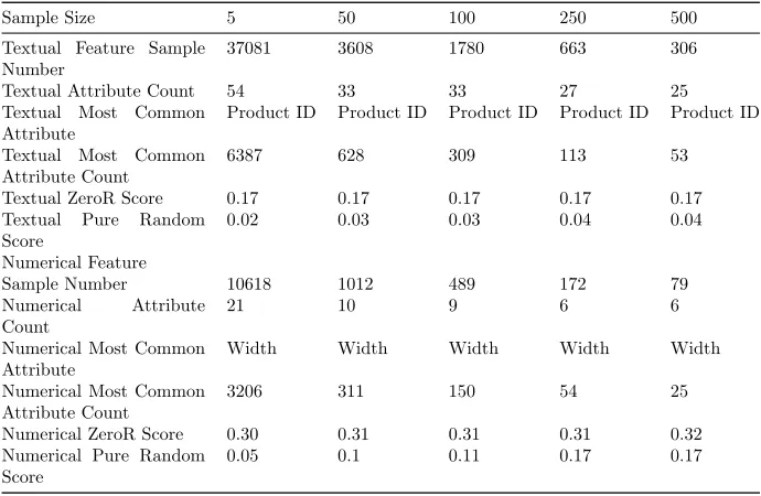
Sample Size 5 50 100 250 500

Textual Score 0.90 0.96 0.97 0.96 0.94

Textual Score Standard Deviation

0.003 0.003 0.002 0.008 0.010

Numerical Score 0.87 0.89 0.88 0.93 0.90

Numerical Score Standard Deviation

0.001 0.003 0.012 0.010 0.015

(38)

Sample Size 5 50 100 250 500

Textual Feature Sample Number

37081 3608 1780 663 306

Textual Attribute Count 54 33 33 27 25

Textual Most Common

Attribute

Product ID Product ID Product ID Product ID Product ID

Textual Most Common

Attribute Count

6387 628 309 113 53

Textual ZeroR Score 0.17 0.17 0.17 0.17 0.17

Textual Pure Random

Score

0.02 0.03 0.03 0.04 0.04

Numerical Feature

Sample Number 10618 1012 489 172 79

Numerical Attribute

Count

21 10 9 6 6

Numerical Most Common Attribute

Width Width Width Width Width

Numerical Most Common Attribute Count

3206 311 150 54 25

Numerical ZeroR Score 0.30 0.31 0.31 0.31 0.32

Numerical Pure Random Score

[image:38.612.133.478.124.349.2]

0.05 0.1 0.11 0.17 0.17

Table 4.2: Metadata results of experiment Full Dataset with randomized sam-ples divided into fixed size groups

Experiment Discussion: When looking at the results of the data we can see several things. Firstly sample size 5 and 500 do not perform as bad as expected but do still perform worse. both of these sample sizes have lower textual scores scores than sample sizes 50, 100, 250 though sample size 500 does have the second highest numerical score. The ZeroR score remains consistent across all sample sizes. There is a small amount of variation due to the sample size acting as a minimum size requirement and not all columns being able to meet this requirement. Between sample size 5 and 50 there is a significant decrease in the number of attributes. This indicates that those attributes do not have any data columns associated with them of a size larger than 50 values. This also means that those attributes are scarcely present. Looking at performance as well as the number of attributes present 50, 100 and 250 as sample sizes perform best. The most common attribute remains the same across all sample sizes which is logical. It seems that roughly 1/6th of the textual data values is product ID and roughly 1/3rd of the numerical data is width data. A potential issue when using this methodology however is that we have relatively few samples to work with.

4.1.2 Full Dataset with fixed size samples created from

resampling the data

(39)

accurate idea of the data and should thus perform poorly. Similarly a too large sample size may provide too few data points.

Experiment Setup: We will process the full Deep Grooved Ball Bearing dataset using our preprocessing steps with the sampleizer set up to generate a fixed number of samples from each data source of fixed size and generating all features. The way each sample is generated is by collecting a random selection of data values equal to the sample size before returning all the collected val-ues to the available pool. This means that within the same sample the same exact entry cannot be repeated but across all samples it may be used several times. We transform the generated features to Unit Standard Deviation. We will train and test the resultant processed data using a 90%/10% training/test split on a machine learner using the nearest neighbour algorithm using default hyperparameters.

Variations in the Experiment: We will test with 100 and 1000 samples being generated For each of those 2 sample counts we will generate samples sizes of 5, 50, 100, 250. and 500. Any Column which does not meet a minimum size equal to the sample size will not generate samples since such column are too small to generate even one sample.

Measurements: For assessing the results of this experiment we will perform the experiment 5 times and utilize the score() function from the machine learner to calculate a mean score and a standard deviation for those scores. To gain an insight into the data we are working with we also collect a number of metadata values. The meta data collected are:

• Attribute Count

• ZeroR Score

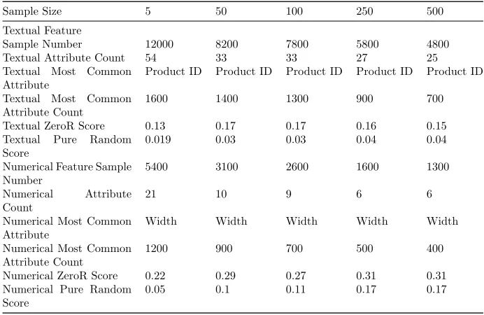
Sample Size 5 50 100 250 500

Textual Score 0.83 0.96 0.98 0.993 0.99

0.006 0.006 0.002 0.001 0.001

Numerical Score 0.79 0.92 0.92 0.91 0.90

0.002 0.004 0.003 0.003 0.004

(40)

Sample Size 5 50 100 250 500

Textual Feature

Sample Number 12000 8200 7800 5800 4800

Textual Most Common

Attribute

Textual Most Common

Attribute Count

1600 1400 1300 900 700

Textual Pure Random

Score

0.019 0.03 0.03 0.04 0.04

Numerical Feature Sample Number

5400 3100 2600 1600 1300

Numerical Attribute

Count

21 10 9 6 6

1200 900 700 500 400

0.05 0.1 0.11 0.17 0.17

Table 4.4: Metadata results of experiment Full Dataset with fixed size samples created from resampling the data for 100 samples.

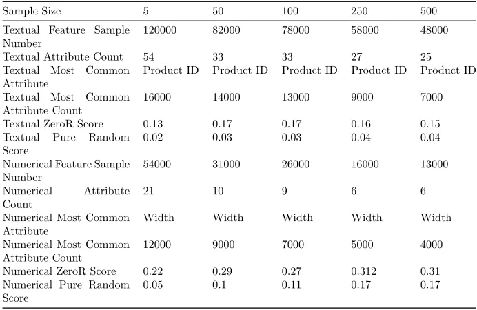
Sample Size 5 50 100 250 500

Textual Score 0.85 0.97 0.98 0.99 0.99

0.006 0.003 0.001 0.002 0.002

Numerical Score 0.81 0.94 0.9 0.92 0.90

[image:40.612.132.478.124.349.2]

0.002 0.001 0.002 0.002 0.002

(41)

Sample Size 5 50 100 250 500

120000 82000 78000 58000 48000

Textual Most Common

Attribute

Textual Most Common

Attribute Count

16000 14000 13000 9000 7000

Textual Pure Random

Score

0.02 0.03 0.03 0.04 0.04

54000 31000 26000 16000 13000

Numerical Attribute

Count

21 10 9 6 6

12000 9000 7000 5000 4000

[image:41.612.132.478.124.349.2]

0.05 0.1 0.11 0.17 0.17

Table 4.6: Metadata results of experiment Full Dataset with fixed size samples created from resampling the data for 1000 samples.

Experiment Discussion: While the final average scores of this method are higher than the earlier data split method we can also note that as the number of samples increase we are having a convergent effect. Examining the ZeroR and the ratio between the number of samples and the most common attribute count shows that this is changing significantly as the sample size increases. Comparing this to the data split method where this ratio (and thus the ZeroR score) was fairly consistent and we did not have as much of a convergent effect it seems likely that we have some distortion due to oversampling. Comparing the generation of 100 and 1000 samples is less significant due to this distortion but overall it seems that generating 1000 samples performs slightly better.

4.1.3 Full Dataset with fixed size samples created from

resampling the data with repeat in the same data

Hypothesis: We expect that different sample sizes should not affect the per-formance of the methodology,however a too small sample size would not give an accurate idea of the data and should thus perform poorly. Similarly a too large sample size may provide too few data points. This specific form of sampling may additionally display quirks in datasets of insufficient size since it is now able to generate such data but the repetition may be too much.

(42)

features. The way each sample is generated is by collecting a random selection of data values equal to the sample size with each data value being available for reuse within the same sample. This means that within the same sample the same exact entry can be repeated as well as across all samples. We transform the generated features to Unit Standard Deviation. We will train and test the resultant processed data using a 90%/10% training/test split on a machine learner using the nearest neighbour algorithm using default hyperparameters.

Variations in the Experiment: We will test with 100 and 1000 samples being generated For each of those 2 sample counts we will generate samples sizes of 5, 50, 100, 250, and 500. Any Column which does not meet a minimum size equal to the sample size will not generate samples since such column are too small to generate even one sample.

Measurements: For assessing the results of this experiment we will perform the experiment 5 times and utilize the score() function from the machine learner to calculate a mean score and a standard deviation for those scores. To gain an insight into the data we are working with we also collect a number of metadata values. The meta data collected are:

• Attribute Count

• ZeroR Score

Sample Size 5 50 100 250 500

Textual Score 0.82 0.96 0.97 0.99 0.99

0.003 0.004 0.005 0.001 0.002

Numerical Score 0.78 0.92 0.92 0.91 0.89

0.002 0.004 0.007 0.003 0.003

(43)

Sample Size 5 50 100 250 500

12000 8200 7800 5800 4800

Textual Most Common

Attribute

Textual Most Common

Attribute Count

1600 1400 1300 900 700

Textual Pure Random

Score

0.02 0.03 0.03 0.04 0.04

5400 3100 2600 1600 1300

Numerical Attribute

Count

21 10 9 6 6

1200 900 700 500 400

0.05 0.10 0.11 0.17 0.17

Table 4.8: Metadata results of experiment Full Dataset with fixed size samples created from resampling the data with repeat in the same data for 100 samples.

Sample Size 5 50 100 250 500

Textual Score 0.84 0.97 0.98 0.99 0.99

0.007 0.003 0.001 0.002 0.000

Numerical Score 0.81 0.94 0.94 0.92 0.90

[image:43.612.132.478.124.349.2]

0.002 0.001 0.001 0.001 0.002

(44)

Sample Size 5 50 100 250 500

120000 82000 78000 58000 48000

Textual Most Common

Attribute

Textual Most Common

Attribute Count

16000 14000 13000 9000 7000

Textual Pure Random

Score

0.02 0.03 0.03 0.03 0.04

54000 31000 26000 16000 13000

Numerical Attribute

Count

21 10 9 6 6

12000 9000 7000 5000 4000

[image:44.612.133.478.124.349.2]

0.05 0.1 0.11 .0.17 0.17

Table 4.10: Metadata results of experiment Full Dataset with fixed size samples created from resampling the data with repeat in the same data for 1000 samples.

Experiment Discussion: Our observations of this experiment shows mostly the same result as the resampling method without reuse and the discussion for that experiment also applies to this experiment.

(45)

4.1.4 Issues found based on the tested sampling methods

Found Issues: Based on the previous experiments we have found several po-tential issues with our current methods of sampling. The current requirements we have set for the data to be considered suitable for use may be incorrect. This manifests itself into a variety of issues:

• When generating samples for the split into fixed group methodology small data samples may generate too few samples meaning that there are is not enough representation of some attributes when creating the training splits.

• In the various resampling methods smaller datasets (not much bigger than the sample size) may result in too much repeat in the sampled data since from that small dataset all generated samples are nearly identical, meaning that scores are artificially inflated and that there is a measure of overtrain-ing.

• This issue with smaller datasets cuts both ways since we are generating the same number of samples regardless of how large each dataset is. Since we are working with multiple datasets each of the same attribute this means that proportionality is lost. While the effect of this is difficult to determine we do feel that maintaining this on some level is important.

Having determined these issues we devised an additional sampling method to alleviate these issues. This method is based on our second sampling method however we have set additional requirements on the minimum size of the dataset as well as an additional limiter on the number of samples that can be created based on the size of the dataset.

4.1.5 Issues found based on the tested sampling methods

Found Issues: Based on the previous experiments we have found several po-tential issues with our current methods of sampling. The current requirements we have set for the data to be considered suitable for use may be incorrect. This manifests itself into a variety of issues:

• When generating samples for the split into fixed group methodology small data samples may generate too few samples meaning that there are is not enough representation of some attributes when creating the training splits.

• In the various resampling methods smaller datasets (not much bigger than the sample size) may result in too much repeat in the sampled data since from that small dataset all generated samples are nearly identical, meaning that scores are artificially inflated and that there is a measure of overtrain-ing.

(46)

means that proportionality is lost. As we are not trying to compensate for distribution of data and even of that case this is a rather unguided method we want to maintain this proportionality.

Having determined these issues we devised an additional sampling method to alleviate these issues. This method is based on our second sampling method however we have set additional requirements on the minimum size of the dataset as well as an additional limiter on the number of samples that can be created based on the size of the dataset.

4.1.6 Full Dataset with fixed size samples created from

resampling the data with additional limiters

When using our new revised method we once again utilize sampling with return-ing the data to the pool once each feature is generated however we have added two additional limiters. For a group of data to be allowed to be sampled it must be at least 2 times the sample size (50 sample size means a minimum dataset size of 100) and to attempt to keep some proportionality a group of data may only be used to generate samples equal to 3 times the dataset size divided by the sample size (in our example of a sample size of 50 with a data group size of 100 this mean 6 samples of 50 each (3*100/50=6)).

Hypothesis: We believe that with these additional limiters the revised sampling method will score worse than the previous resampling methods but that this will mainly be due to the fact that the previous resampling methods were working with distorted sample data resulting in artificially higher scores. This revised method should perform roughly similar to the data split method but should be more robust than that methodology due to the resampling.

Experiment Setup: We will process the full Deep Grooved Ball Bearing dataset using our preprocessing steps with the sampleizer set up to generate a fixed number of samples from each data source of fixed size and generating all features. The way each sample is generated is by collecting a random selection of data values equal to the sample size before returning all the collected val-ues to the available pool. This means that within the same sample the same exact entry cannot be repeated but across all samples it may be used several times. We transform the generated features to Unit Standard Deviation. We will train and test the resultant processed data using a 3 fold cross validation on a machine learner using the nearest neighbour algorithm with grid searching hyperparameters for each uneven amount of neighbours from 1 to 31 and using .euclidean or minkowski distance metrics.

Variations in the Experiment: We will test with 100 and 1000 samples being generated. For each of those sample numbers we will generate samples sizes of 5, 50, 100, 250, and 500.

(47)

insight into the data we are working with we also collect a number of metadata values. The meta data collected are:

• Attribute Count

• ZeroR Score

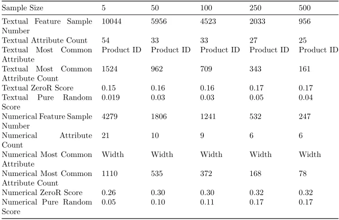
Sample Size 5 50 100 250 500

Textual Score 0.83 0.95 0.97 0.99 0.99

0.011 0.005 0.006 0.004 0.007

Numerical Score 0.77 0.83 0.86 0.91 0.90

.0071 0.017 0.014 0.020 0.032

(48)

Sample Size 5 50 100 250 500

10044 5956 4523 2033 956

Textual Most Common

Attribute

Textual Most Common

Attribute Count

1524 962 709 343 161

Textual Pure Random

Score

0.019 0.03 0.03 0.05 0.04

4279 1806 1241 532 247

Numerical Attribute

Count

21 10 9 6 6

1110 535 372 168 78

0.05 0.10 0.11 0.17 0.17

Table 4.12: Metadata results of experiment Full Dataset with fixed size samples created from resampling the data with additional limiters for 100 samples.

Sample Size 5 50 100 250 500

Textual Score 0.88 0.97 0.97 0.99 0.99

0.005 0.003 0.004 0.005 0.004

Numerical Score 0.80 0.88 0.88 0.91 0.91

[image:48.612.132.478.124.349.2]

0.004 0.011 0.011 0.022 0.031

(49)

Sample Size 5 50 100 250 500

61525 10917 5413 2033 956

Textual Most Common

Attribute

Textual Most Common

Attribute Count

9763 1900 939 343 161

Textual Pure Random

Score

0.02 0.03 0.03 0.04 0.04

19309 3058 1484 532 247

Numerical Attribute

Count

21 10 9 6 6

5580 938 453 168 78

[image:49.612.133.478.124.349.2]

0.05 0.10 0.11 0.17 0.17

Table 4.14: Metadata results of experiment Full Dataset with fixed size samples created from resampling the data with additional minimals and maximals for 1000 samples.

(50)

4.1.7 Graphical Comparison between sampling methods

To improve the readability and aid in the comparison of the various methods we have generated a number of graphs from the tabulated scores of each sampling method.

(51)

Figure 4.2: Graph of the textual scores for all previous sampling experiments.

Automatic instance based matching of database schemas of web harvested product data

University of Twente