University of Warwick institutional repository: http://go.warwick.ac.uk/wrap
A Thesis Submitted for the Degree of PhD at the University of Warwick
http://go.warwick.ac.uk/wrap/58125
This thesis is made available online and is protected by original copyright. Please scroll down to view the document itself.
Elmedin Selmanovi´
c
BSc (Hons)
A thesis submitted for the degree of Doctor of Philosophy in Engineering
School of Engineering University of Warwick
Acknowledgements x
Declaration xi
Abstract xii
1 Introduction 1
1.1 Digital Imaging Pipeline . . . 1
1.1.1 Capture . . . 2
1.1.2 Storage . . . 3
1.1.3 Display . . . 4
1.1.4 Other Techniques . . . 4
1.2 Stereoscopic Imaging . . . 4
1.3 High Dynamic Range Imaging . . . 7
1.4 Research Objectives . . . 10
1.5 Thesis Outline . . . 11
2 Stereoscopic Imaging 13 2.1 A Brief History of Stereoscopy . . . 14
2.2 Theory of Stereo Vision . . . 18
2.2.1 Epipolar Geometry . . . 18
2.2.2 Fundamental Matrix . . . 20
2.2.3 Image Rectification . . . 21
2.2.4 Disparity Maps . . . 21
2.2.5 Stereo Correspondence Algorithms . . . 25
2.3 Visual Discomfort in Stereo Vision . . . 31
2.3.1 Individual Differences . . . 31
2.3.2 Excessive Screen Disparity . . . 32
2.3.3 Vergence - Accommodation Decoupling . . . 32
2.3.4 Zone of Comfortable Viewing . . . 33
2.3.5 Stereoscopic Impairments . . . 34
2.4 Stereoscopic Capture . . . 36
2.4.1 Capturing Two Symmetric Views . . . 37
2.4.4 Stereoscopic Rendering . . . 48
2.5 Stereoscopic Content Storage . . . 49
2.5.1 Animated Graphics Interchange Format (GIF) . . . 50
2.5.2 Stereoscopic Portable Network Graphics Format (PNS) . . 51
2.5.3 Stereoscopic JPEG (JPS) . . . 51
2.5.4 Multiview Video Format (MVC) . . . 52
2.6 Stereoscopic Displays . . . 53
2.6.1 Direct-View Stereoscopic Displays . . . 53
2.6.2 Head-Mounted Displays . . . 55
2.6.3 Autostereoscopic Displays . . . 56
2.7 Summary . . . 58
3 High Dynamic Range Imaging 59 3.1 Theory of High Dynamic Range Imaging . . . 60
3.2 High Dynamic Range Capture . . . 62
3.2.1 Multiple Exposures . . . 63
3.2.2 Native HDR Capture . . . 68
3.2.3 Expansion Operators (EOs) . . . 71
3.3 High Dynamic Range Content Storage . . . 78
3.3.1 File Formats . . . 78
3.3.2 High Dynamic Range Image Coding . . . 84
3.3.3 High Dynamic Range Video Coding . . . 90
3.4 HDR Display . . . 96
3.4.1 Native HDR Displays . . . 96
3.4.2 Tone Mapping . . . 101
3.5 Summary . . . 106
4 Stereoscopic High Dynamic Range Pipeline 107 4.1 SHDR Capture . . . 107
4.2 SHDR Storage . . . 110
4.3 SHDR Display . . . 111
4.4 Summary . . . 112
5 Stereoscopic High Dynamic Range Images 113 5.1 LDR to HDR methods . . . 114
5.1.1 Expansion Operators . . . 116
5.1.2 Stereo Correspondence . . . 117
5.2 The Experiment . . . 121
5.2.1 Methodology . . . 122
5.2.2 Participants . . . 125
5.2.3 Materials . . . 125
5.2.4 Procedure . . . 127
5.3 Results . . . 128
5.3.3 Image Quality Comparison . . . 132
5.4 Discussion . . . 132
5.4.1 Limitations . . . 136
5.5 Summary . . . 137
6 Stereoscopic High Dynamic Range Video 138 6.1 LDR to HDR Methods . . . 139
6.1.1 Stereo Correspondence . . . 139
6.1.2 Expansion Operator . . . 141
6.1.3 Hybrid Method . . . 143
6.2 Results . . . 147
6.2.1 Materials . . . 147
6.2.2 Objective Quality Measurements . . . 149
6.2.3 Qualitative Results . . . 151
6.3 Discussion . . . 151
6.3.1 Limitations . . . 154
6.4 Summary . . . 154
7 Stereoscopic High Dynamic Range Compression 159 7.1 JPEG SHDR Methods . . . 160
7.1.1 Side-by-side (SBS) Method . . . 161
7.1.2 Half Side-by-side (HSBS) Method . . . 162
7.1.3 Image Plus Disparity (IPD) Method . . . 163
7.1.4 Image Plus Disparity with Corrections (IPDC) Method . . 164
7.1.5 Motion Compensation (MC) Method . . . 166
7.2 Results and Analysis . . . 167
7.3 Summary . . . 171
8 Conclusions 174 8.1 Capture of Stereoscopic High Dynamic Range Images . . . 174
8.2 Capture of Stereoscopic High Dynamic Range Video . . . 175
8.3 Compression of Stereoscopic High Dynamic Range Images . . . . 176
8.4 Contributions . . . 178
8.5 Impact . . . 178
8.6 Future Work . . . 179
8.6.1 Extended User Studies . . . 179
8.6.2 Additional Operators . . . 180
8.6.3 SHDR Display . . . 180
8.6.4 Beyond SHDR Imaging . . . 181
8.7 Final Remarks . . . 182
References 183
1.1 Digital Imaging Pipeline . . . 2
1.2 Stereoscopic Imaging . . . 5
1.3 High Dynamic Range Imaging . . . 8
2.1 Wheatsone’s Mirror Stereoscope . . . 16
2.2 Random-dot Stereogram . . . 17
2.3 Illustration of Stereo Capture Setup . . . 19
2.4 Epipolar Geometry . . . 20
2.5 Disparity Map . . . 22
2.6 Keystone Distortion . . . 35
2.7 Single Lens Stereo Camera Setup . . . 38
2.8 Hybrid Stereoscopic Camera . . . 39
2.9 Using Photographs to Enhance Videos . . . 42
2.10 Kinect . . . 45
2.11 Multiview Video Coding . . . 52
2.12 Stereoscopic Glasses . . . 54
2.13 Two-View Autostereoscopic Displays . . . 57
3.1 Dynamic Range . . . 61
3.2 Multiple Exposures . . . 64
3.3 Multiple Exposure Video . . . 67
3.4 HDR Video Camera . . . 70
3.5 Banding Artefact . . . 74
3.6 Overview of the Expand Map Algorithm . . . 76
3.7 Radiance File Format . . . 80
3.8 LogLuv File Format . . . 81
3.9 OpenEXR File Format . . . 83
3.10 JPEG-HDR Encoding Pipeline . . . 85
3.13 Rate-Distortion Optimised HDR Video Encoding Pipeline . . . . 93
3.14 HDR Stereoscopic Viewer . . . 97
3.15 SHDR Viewer Transparency Generation . . . 98
3.16 HDR Projector Based Display . . . 99
3.17 HDR LED Display . . . 100
5.1 Expansion Operator SHDR Method for Images . . . 114
5.2 Stereo Correspondence SHDR Method for Images . . . 115
5.3 COGC Algorithm Artefacts . . . 120
5.4 SHDR Images Used for Testing . . . 126
5.5 Experimental Setup . . . 127
5.6 Preferences of SHDR Methods for Images . . . 130
5.7 Example Images Generated Using SHDR Methods . . . 133
5.8 Comparison of Generated SHDR Images . . . 135
6.1 Generation of SHDR video from HDR-LDR video pair . . . 138
6.2 HDR-LDR Stereo Correspondence Pipeline . . . 140
6.3 HDR-LDR Expansion Operator Pipeline . . . 142
6.4 HDR-LDR Hybrid Pipeline . . . 143
6.5 Disparity Map Generation for SHDR Video . . . 144
6.6 Interpolated Disparity Map . . . 145
6.7 SAD Frame Warping Artefacts . . . 146
6.8 SHDR Video Scenes . . . 148
6.9 SAD Video Method Artefacts . . . 152
6.10 Example Frames Generated Using SHDR Video Methods . . . 155
6.11 Quality Comparison of SHDR Video Frame . . . 156
6.12 PSNR Results for SHDR Video . . . 157
6.13 TQ Results for SHDR Video . . . 158
7.1 SBS Encoding . . . 161
7.2 SBS Decoding . . . 161
7.3 HSBS Encoding . . . 162
7.4 HSBS Decoding . . . 162
7.5 IPD Encoding . . . 163
7.6 IPD Decoding . . . 163
7.7 IPDC Disparity Example . . . 165
7.8 IPDC Disparity Generation . . . 165
7.11 An Example Decoded Image . . . 168 7.12 SHDR Scenes Used for Compression Evaluation . . . 172 7.13 SHDR Scenes Used for Compression Evaluation Continued . . . . 173
5.1 Example Preference Table . . . 123
5.2 Ranking of SHDR Method for Images and the Summary of Results 129 5.3 PSNR Results for SHDR Image Generation . . . 131
5.4 RMSEL Results for SHDR Image Generation . . . 132
6.1 SHDR Video Data . . . 149
6.2 Summary of PSNR Results for SHDR Video . . . 150
6.3 Summary of TQ Results for SHDR Video . . . 151
7.1 SHDR Compression Compatibility . . . 167
7.2 Sizes of Compressed SHDR Images . . . 169
7.3 PSNR Results for SHDR Image Compression . . . 170
7.4 RMSEL Results for SHDR Image Compression . . . 171
7.5 Compression Results Summary . . . 171
Firstly, I would like to thank my supervisors Alan and Kurt. Alan provided me with the opportunity to do a PhD, and his constant support, advice, encourage-ment and enthusiasm are sincerely appreciated. Kurt was a great encourage-mentor who patiently guided me on my PhD path and helped me avoid the many perils of research. Moreover, Kurt was also a true friend and ensured my stay in the UK was enjoyable.
Jasminka and Selma recommended me to Alan, and for this I am very grateful. The members of the Visualisation Group at Warwick University have made the PhD experience exciting and interesting, both professionally but also as friends. Vedad made the transition from Bosnia to England much easier and set me on the right footing. Tom took the role of a third mentor and we had many useful discussions. Carlo, Jass and Vibhor provided a continuous support and offered helpful advice. It was great working with Alena, Alessandro, Ali, Belma, Jon, Josh, Keith, Louis Paulo, Martinho, Miguel, Piotr, Ratnajit, Remi, Sam, Sandro, Silvester, Stratos, Tim and Vasu.
I am also grateful to people outside the group who made life during the PhD fun: Ado, Adnan and Tarik, Alex, Anna, Ammar, Dˇzidˇzo, Jo, Jason, Kate, Mike, Mirza, Mosh and Nedim. I would like to say thank you to everyone I have missed or not mentioned, as there were many others who helped me in numerous ways during the past four years.
My family was there for me throughout the whole time. My grandmas were especially inspiring . Majka Sena demonstrated how persistence and courage can overcome any obstacle while majka Zilha and me shared some of the toughest moments of our lives.
I would like to thank Silvija for providing extra motivation to finish the thesis and for being so loving, patient and supportive. Volim te!
My eternal gratitude goes to my parents Azra and Senad who always made sure I was on the right path and this thesis is the result of such efforts. Hvala!
The work in this thesis is original and no portion of this work has been submitted in support of an application for another degree or qualification at this university or at another university or institution of learning.
Elmedin Selmanovi´c
Two modern technologies show promise to dramatically increase immersion in virtual environments. Stereoscopic imaging captures two images representing the views of both eyes and allows for better depth perception. High dynamic range (HDR) imaging accurately represents real world lighting as opposed to traditional low dynamic range (LDR) imaging. HDR provides a better contrast and more natural looking scenes. The combination of the two technologies in order to gain advantages of both has been, until now, mostly unexplored due to the current limitations in the imaging pipeline. This thesis reviews both fields, proposes stereoscopic high dynamic range (SHDR) imaging pipeline outlining the challenges that need to be resolved to enable SHDR and focuses on capture and compression aspects of that pipeline.
The problems of capturing SHDR images that would potentially require two HDR cameras and introduce ghosting, are mitigated by capturing an HDR and LDR pair and using it to generate SHDR images. A detailed user study compared four different methods of generating SHDR images. Results demonstrated that one of the methods may produce images perceptually indistinguishable from the ground truth.
Insights obtained while developing static image operators guided the design of SHDR video techniques. Three methods for generating SHDR video from an HDR-LDR video pair are proposed and compared to the ground truth SHDR videos. Results showed little overall error and identified a method with the least error.
Once captured, SHDR content needs to be efficiently compressed. Five SHDR compression methods that are backward compatible are presented. The proposed methods can encode SHDR content to little more than that of a traditional single LDR image (18% larger for one method) and the backward compatibility property encourages early adoption of the format.
The work presented in this thesis has introduced and advanced capture and compression methods for the adoption of SHDR imaging. In general, this research paves the way for a novel field of SHDR imaging which should lead to improved and more realistic representation of captured scenes.
Keywords: Stereoscopy, High Dynamic Range
Introduction
Humans rely extensively on visual information to interpret the surrounding en-vironment. Presenting the human visual system (HVS) with captured or created data which is indistinguishable from reality remains one of the main goals of dig-ital imaging. Established techniques are able to convey the impression of a real scene, to an extent, but are still limited in a number of aspects including accu-rate light and depth reproduction. More recent digital techniques such as high dynamic range (HDR) imaging and stereoscopic imaging are able to overcome some of these limitations. More specifically, HDR imaging is able to preserve the full range of light available in the scene, thereby improving representation of light in an image, while stereoscopic imaging improves depth perception by simulating binocular vision (observing the world with both eyes). Each of these methods comes with a number of challenges which, so far, have been explored in isolation. This thesis brings HDR imaging and stereoscopic imaging together, and tackles some of the problems that arise as a result of this integration. It proposes a novel imaging method which advances current imaging technology.
1.1
Digital Imaging Pipeline
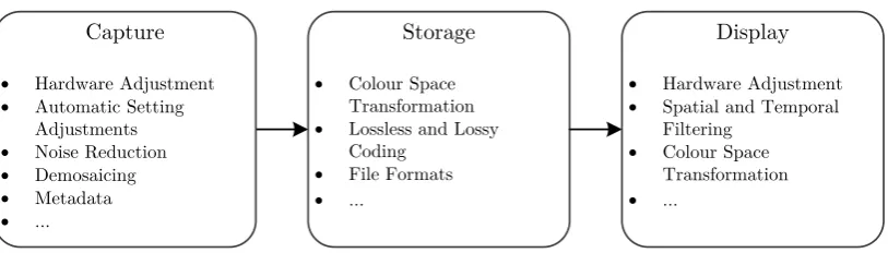
As this thesis is dealing with a new imaging method, the general imaging pipeline needs to be introduced. Any image or video passes through a number of ma-nipulations in its lifetime. In general, this can be seen to consist of three key stages: capture, storage and display. They constitute the digital imaging pro-cessing pipeline, as is shown in Figure 1.1. Each stage of the traditional pipeline contains a set of established functions and operations which modify the content depending on the intended application. Each stage is examined in more detail
Storage
· Colour Space Transformation
· Lossless and Lossy Coding
· File Formats
· ...
Capture
· Hardware Adjustment
· Automatic Setting Adjustments
· Noise Reduction
· Demosaicing
· Metadata
· ...
Display
· Hardware Adjustment
· Spatial and Temporal Filtering
· Colour Space Transformation
[image:15.595.117.524.105.221.2]· ...
Figure 1.1: The digital imaging pipeline represents the stages through which images and videos pass from capture to display. In each stage different processing steps may be applied depending on the intended application.
in the next sections. Focus is placed on capture and compression, as the thesis contributes to these two stages.
1.1.1
Capture
Capture is concerned with recording images and videos. One aspect of this is the specification and choice of the right hardware which includes optics, sensors and lights. The skill of the device operator may be crucial, as visual data not recorded properly may be lost. The next important aspect is quality of the sensor as it determines key properties of the captured image or video: the resolution, amount of noise, quality of colour representation, dynamic range, sharpness and number of recorded frames.
may also contain metadata, which gives image or video properties. This can be useful in later stages of the pipeline (e.g. using exposure value metadata for creating HDR images).
Finally, content may also be generated using computer graphics. Setting up a virtual scene may require significant user input. Objects need to be modeled, textured, animated and rendered. While it may be time consuming, the output is usually of high quality.
1.1.2
Storage
It is common for colour images to consist of three colour channels: red, green and blue. Each of the channels is typically represented by a single byte which totals approximately 6.2 MB for a full high definition (HD) image (resolution
of 1920×1080) or around 186 MB for each second of HD video captured at 30
frames per second (fps). However, most of the pixels are highly correlated so it can be expected that neighbouring pixels are similar to each other. In video, the changes between consecutive frames are usually small, meaning that pixels at the same spatial position are likely correlated. These facts allow for compression (encoding) methods which can reduce file sizes significantly.
Two general types of encoding exist: lossless and lossy. Lossless uses com-pression techniques which reduce redundancy and which are, also, fully reversible. Decoded content is identical to the original as all the data is preserved. Higher compression rates may be achieved by sacrificing some information resulting in lossy coding. The characteristics of the HVS and human perception are utilised in these approaches and data which is deemed less perceptually important is eliminated. This results in images or videos which are different from the original, but these differences - depending on the amount of compression - should not be noticeable to an observer. At this stage, the image may be converted to a differ-ent colour space which decorrelates colours better, improving compression. Also, improvements may be achieved by downsampling less influential channels. Both encoding and decoding may require substantial processing time which is not ac-ceptable for real-time applications. To overcome this hardware implementations of standard techniques exist.
to open and display any content that follows an agreed specification irrespective of the encoding technique used.
1.1.3
Display
The final stage of the imaging pipeline is display and it relies heavily on hard-ware. Many manufacturers use custom processing methods to improve video reproduction on their devices. This includes contrast boosts and spatial filter-ing to improve appearance. Devices themselves may use different colour spaces requiring appropriate transformations. The screen resolution is typically fixed while it can receive content of many different sizes. Upsampling and downsam-pling may be required in such cases ensuring the image is displayed properly on the screen.
1.1.4
Other Techniques
In addition to these stages, the image may be manipulated in other ways by different applications. Compositing is a technique used in visual effects where parts of multiple images and/or videos are combined into a single one. Different filters may be applied to change the look and feel of the image, frequently for artistic purposes. For instance, an image may be turned from colour to greyscale and noise might be added to achieve an antique appearance. In-painting allows unwanted objects to be removed from the images and videos, by filling the empty regions with surrounding content.
1.2
Stereoscopic Imaging
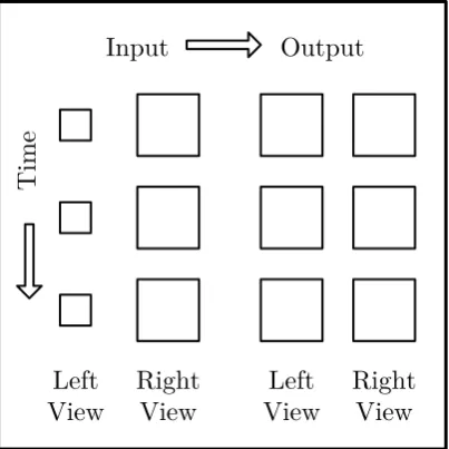
Stereoscopic imaging enhances the perception of depth using two binocular depth cues: stereopsis and vergence (see Figure 1.2). Stereopsis is the phenomenon in which points in the observed environment project to different locations on the retina based on their distance from the observer. Vergence is the movement of the eyes to or from each other which ensures that the object of interest is projected to the centre of the retina. The distance of the focused object determines the angle of vergence which is used to infer depth.
(a) Left View (b) Right View
[image:18.595.115.529.95.481.2](c) Depth Perception
Figure 1.2: In binocular vision each eye gets slightly different view of the world. HVS uses discrepancies between the views to infer depth of the scene. Depth sensation is visualised in image (c) where brighter values represent closer objects. Completely black regions are occluded and cannot be seen by one of the eyes. Images courtesy of Scharstein & Szeliski (2003).
specific positions so that each eye gets its intended view.
A vast amount of research has compared stereoscopic to traditional two-dimensional viewing and a number of literature surveys are available. McIntire
et al. (2012) reviewed and classified 71 objective experiments which examined human performance of 2D versus 3D displays. Overall results showed that 58% of the experiments found that 3D benefited measured human performance, 14% offered mixed results, while 28% showed no improvement in performance. There-fore 72% of the experiments demonstrated at least some benefit of stereo displays. Experiments were categorised into 6 groups based on performance type: (1) po-sition and distance judgement, (2) identifying objects, (3) spatial manipulation of objects, (4) navigation, (5) spatial understanding and (6) learning. The ma-jor benefit of stereo displays was apparent for spatial understanding and spatial manipulation tasks (92% and 85% respectively, showed at least some benefit). Only two studies were examined in the learning category and they showed a lack of improvement. The other three categories had approximately half the experiments showing some benefit. This review excluded medical related liter-ature because satisfactory summaries already exist. For instance, Held & Hui (2011) examined how 3D displays could improve diagnostic, surgery and train-ing in medicine. They concluded that displays could: help doctors in detecttrain-ing diagnostically relevant anatomical features, help novice surgeons in navigating the surgical landscape and aid in performing complicated tasks, and help stu-dents with anatomical understanding. Similarly, Getty & Green (2007) focused on medical applications and presented five cases where stereo displays were suc-cessfully used: teaching anatomy, digital mammography, tomography, diabetic retinopathy and minimal invasive surgery.
A literature review for military applications was provided by Dixon et al. (2009) who were concerned with displaying complex information using stereo and perspective representations, and they summarised 75 relevant papers. They concluded that 3D technology was the most useful in representing qualitative information, providing a quick overview of data, facilitating mission rehearsal, helping in route planning, visualising network attacks and providing realistic simulator training.
esti-mating firmness of salmon fillets.
Chapter 2 provides an overview of stereoscopic imaging. It provides a short history of the field, describes important theoretical concepts and examines how challenges at each stage of the imaging pipeline are being tackled.
1.3
High Dynamic Range Imaging
Current imaging techniques - termed low dynamic range (LDR) - are able to
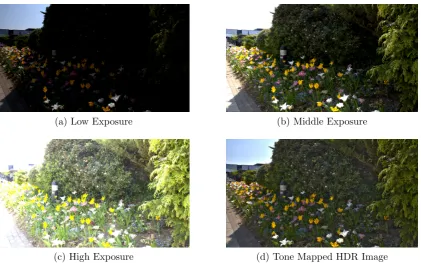
capture only a limited dynamic range. This causes overexposed (white) and un-derexposed (black) regions in an LDR image at the places which would otherwise contain details. For example, when taking photograph of a sunny day, one has to choose between capturing either the background sky and highlights or cap-turing the details in the shadow, even though both are visible to the observer, as illustrated in Figure 1.3. High dynamic range (HDR) imaging overcomes this limitation and is able to preserve the full range of light available in a scene.
High dynamic range imaging enhances the quality of image colour reproduc-tion (Reinhard et al., 2010), and as such it inherently provides benefits to many fields which rely on digital images and which are not hindered by image size. HDR imaging is also useful in a number of other more direct application areas.
Physically based rendering was one of the first applications for HDR imaging. In order to simulate light transport accurately, rendering programs need to store and process the full dynamic range of light (Ward, 1994a) and the final output may be scaled to match traditional formats using tone-mapping techniques (Ban-terleet al., 2011). Increased precision is another useful property of HDR relevant for physically based rendering as it prevents error accumulation in multi-stage, multi-pass algorithms. HDR environment maps are used for image-based lighting, where HDR captured real-world lighting is used to light a virtual scene, thereby improving the realism and quality of the generated image.
Remote sensing acquires information about a phenomenon or an object with-out physical contact. Frequently, it refers to an aerial sensor detecting and classi-fying objects on Earth. Images captured using such an approach usually contain data outside human visible range (Lillesandet al., 2004), making HDR of special importance for this application area.
(a) Low Exposure (b) Middle Exposure
[image:21.595.112.534.107.370.2](c) High Exposure (d) Tone Mapped HDR Image
Figure 1.3: When capturing a scene which contains a wide range of light with current hardware one needs to chose whether to lose details in highlights or in shadows. (a) When capturing low exposure it is possible to see information in highlights, but the rest of the detail is lost. For example, the colour of the sky is visible. (b) Middle exposure provides a tradeoff by clipping the image both in the highlights and shadows but it preserves most of the data. (c) High exposure contains all shadow details but the rest of the image is overexposed. (d) The combination of the three exposures into a single HDR image which preserves all the information visible to the human eye.
which wants to use them needs to implement each one individually. This pro-cess is cumbersome, inconvenient and reduces compatibility. An elegant solution would use HDR as the standard encoding, which will likely become the case in the future. A downside of such an approach might be the file size, but top end consumer cameras already use 16 bits per channel for the RAW representation which could be used to represent HDR data instead.
steps - a problem avoided by using HDR.
The entertainment industry is starting to recognise the potential of HDR. The current trend in digital cinema and the movie industry is turning towards medium dynamic range for digital film distribution. The main challenge which prevents HDR entering the mainstream is file-size. The development of robust and efficient compression algorithms will likely overcome this problem and HDR video may eventually reach the home screen. Many computer game engines render in HDR and tone-map output for increased realism. HDR texture compression is also becoming a critical element in the game rendering pipeline (Munkberget al., 2008).
Virtual reality (VR) strives to provide a realistic rendition of the real world which requires a true light representation and simulation. The HDR requirement for VR applications is highlighted by the fact that users may move around a virtual space that contains sharp light changes (e.g. walking from inside to the outside of a house).
Computer vision extracts information from photographs or video which can help solve a number of tasks including robot navigation, event detection, infor-mation organization and automatic inspection. HDR images provide more data and may improve performance of many computer vision algorithms. For example, Cui et al. (2011) suggest a method for generating reliable material colour images by subtracting highlights and shadows, which are recognised with the the help of HDR data. If the algorithm is required to run in real time, the HDR data size might become an issue.
Security systems which rely on video monitoring may benefit from HDR. Security cameras are frequently positioned to observe entrances of buildings or windows. Such a setup is especially susceptible to sharp differences in contrast, where the inside of the building is expected to be dark with strong shadows while outside may be bright and sunny. Traditional cameras would have to choose which of the two extremes will be filmed, or worse they might auto adjust to the middle range and risk capturing everything poorly. In addition, traditional cameras have problems with dark environments which are usually recorded with an increased amount of noise - and which are, in terms of security, usually more important. Future HDR cameras are expected to perform well in both setups.
especially the case for professions such as medical surgery. Here operations are performed under strong lights which focus on specific regions thereby creating sharp contrast.
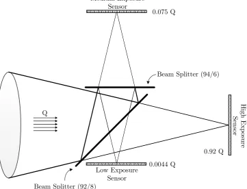
Switching from traditional LDR to HDR imaging requires alterations to and optimisation of the imaging pipeline. Sensors which capture such a range with all the colours and with satisfactory resolution have not been designed yet. To overcome this, multiple images of the same scene may be taken at different ex-posures and combined. Such an approach is not feasible for video due to a speed requirement. Instead multiple sensors and a beam splitter (optical elements that let some amount of light pass and reflect the rest) are aligned so that a differ-ent amount of light arrives at each of the sensors, after which the images are combined. The amount of HDR data is quadrupled compared to LDR imaging as data is represented by floating point numbers which use 4 bytes per colour channel instead of a single byte as is the case with LDR data. Lossy methods which achieve high compression rates have been proposed and try to quantise the image so that errors are not perceivable by the HVS. The problem of con-structing displays which would enable natural visualisation of HDR content has been tackled as well. The current solutions rely on a combination of a low res-olution LED array which boosts the range and a standard LCD display which reproduces details. Alternatively, the range of HDR content may be scaled down and displayed on LDR screens - a technique termed tone mapping.
High dynamic range imaging is an active research area and is reviewed in more detail in Chapter 3. Theoretical concepts behind HDR imaging are described, and proposed methods and algorithms that tackle problems at each stage of the pipeline are examined.
1.4
Research Objectives
The combination of stereoscopic and high dynamic range imaging has been, until now, mostly unexplored. This thesis aims to merge these techniques in order to create a powerful visualisation method, building upon the existing knowledge in both areas. The main research objectives of this thesis are:
to recognize the potential challenges that arise from the merge of stereo-scopic and HDR technologies
to devise and validate an approach which facilitates capturing of SHDR
images and overcomes limitations posed by using two static HDR cameras
to propose and validate a temporally robust approach for capturing SHDR videos using insights gained while developing techniques for single images
to devise and evaluate techniques for compressing SHDR images which
are backwards compatible with traditional imaging techniques and thereby facilitate the adoption of SHDR imaging
1.5
Thesis Outline
This thesis consists of eight chapters, which are arranged as follows:
Chapter 2: Stereoscopic Imaging: Provides an overview of stereoscopy with a focus on concepts relevant to this thesis. This chapter presents a brief history of stereoscopy, explores important theoretical aspects such as epipo-lar geometry and disparity maps, examines visual comfort, and covers the stereoscopic imaging pipeline (capture, storage and display).
Chapter 3: High Dynamic Range Imaging: Examines the main concepts of high dynamic range imaging which are relevant for this thesis. It fo-cuses on the HDR imaging pipeline (capture, storage and display).
Chapter 4: Stereoscopic High Dynamic Range Imaging Pipeline: Explains the different stages of SHDR image and video processing. It presents chal-lenges which need to be addressed to enable SHDR.
Chapter 5: Generating SHDR Images using an HDR-LDR Camera Pair:
Chapter 6: Generating SHDR Video using HDR-LDR Camera Pair: The approach which performed the best for obtaining SHDR images is extended to enable video capture. Achieving temporal constancy is challenging re-quiring techniques which prevent flickering. The proposed techniques are compared to the best static one.
Chapter 7: SHDR Coding: Proposes and compares five image coding meth-ods. Two methods format images so that existing coders can be used, two methods exploit disparity maps while the last one relies on motion com-pensation to compress differences.
Stereoscopic Imaging
The ultimate goal of computer graphics is to obtain a realistic representation of the imaged scene to be viewed by people. The main purpose of the human visual system (HVS) is the inverse - to infer the geometric properties of the observed environment and extract information about events, objects and location. One key ability of the HVS is to perceive depth, as this allows understanding of the world in three dimensions. It is therefore desirable that captured video and images are able to correctly represent such characteristics.
Depth cues can be divided into two groups: monocular and binocular (Gold-stein, 2009). Monocular cues are observed by one eye and are used in traditional media (e.g. paintings and photographs). They include: perspective, relative size, familiar size, occlusion, texture gradient, defocus blur and accommodation. Binocular depth cues, which use both eyes, are stereopsis and vergence.
Objects in the environment project to different positions on a retina based on how far they are from the observer. The HVS uses this information to infer depth, in a phenomenon termed stereopsis or binocular vision. When inspecting the object of interest, eyes move to or from each other, to project it onto the centre of the retina. This simultaneous horizontal movement is called vergence.
Stereoscopy is any imaging technique which enhances or enables depth per-ception using the binocular vision cues. The following subsections examine a brief history and theory of stereoscopy, discuss potential viewing discomfort, and present its imaging pipeline with special focus on disparity map generation.
2.1
A Brief History of Stereoscopy
It is interesting that mechanisms of stereopsis were understood only around 170 years ago while the required theory was attainable since ancient times. Greek philosophers were the first to recognize the problem of perceiving a single image
while observing the world with two eyes - a phenomenon termed singleness of
vision. Aristotle (384 - 322 BC) noticed how the image of the viewed object doubled, by pressing an eye. In about 300 BC, Euclid wrote the earliest known book on optics simply titledOptics which contained over 60 theorems relevant to this day. He observed that the world appears somewhat different when viewed by each eye. Euclid, like many Greek philosophers, adhered to the emission theory
of light - suggested by Empedocles (5th century BC) - which stated that rays of light left an eye in a cone shape and sensed the surface on which they fell, like fingers. Ptolemy (127 - 165) thoroughly investigated binocular vision but was concerned with the singleness of vision, and not depth perception. He also followed emission theory and stated that axes of ray cones, projected from an eye, are the lines of fixation. When the lines meet on an object it is seen as one. Then he mistakenly concluded that the single vision in periphery is achieved for the points lying on a frontal plane passing through the fixation point. Had he chosen the circle passing through the fixation point and centre of the eyes instead (which he had the idea of), he would have come to the modern definition of horopter: a set of points in space that get fused into a single vision. Also he mistakenly believed that the eye could sense distance from the length of the ray projected from the eye to the object. Galen (AD 129 - 201), too, tackled the problem of single vision. He suggested that it occurs at the crossing of optic nerves (chiasm) where two images unite. Galen also noticed that near objects during binocular vision appeared at two different places in the background.
enters and forms an inverted image. Following Ptolemy, Alhazen explained that objects near intersection of lines of fixation appear single, but also added that other objects to the side of the frontal plane double. Even though he realised that horopter was not corresponding to the frontal plane, he did not go a step further and show it was actually a circle. In terms of depth perception Alhazen was focused on monocular cues such as apparent size, aerial perspective and parallax during head motion; but he also made an important contribution to binocular depth perception: recognising that we could sense a degree of convergence of the eyes.
Further major advances in knowledge about binocular vision occurred in sev-enteenth century. Before this, Leonardo da Vinci and Giovanni Battista della Porta (1535 - 1615) also made contributions; Leonardo analyzed partial and to-tal occlusions and noted their role in depth perception while Giovanni reported the phenomenon of binocular rivalry when observing different images with each eye. In 1613, Franciscus Aguilonius published a book on optics, synthesizing the works of Euclid, Alhazen, Vitello and and others. He understood that binocu-lar vision improved depth perception, and coined the term horopter but used it differently to its modern meaning. For him the horopter was the frontal plane passing through the convergence point where all vision rays ended, leading to sin-gle or double vision. Aguilonius also rejected Alhazen’s proposal of convergence as a cue for distance, but introduced a new important idea: the length of the ray of one eye can be judged by the other.
Johannes Kepler (1571 - 1630) set the first geometrical principles of image formation in the eye. He noted that an image of the outer world projected on the retina is inverted and flat. This discovery made the problem of stereopsis harder by posing the question of how depth can be seen from flat images. Kepler’s solution was the same as Alhazen’s: we perceive distance by sensing the rotation of the eyes. In 1667, Christiaan Huygens defined corresponding retinal points -the points in each eye that have -the same location in relation to -the centre of the retina. Isaac Newton, incorrectly, presumed that fibres from corresponding retinal points fuse in chiasma (the place where optic nerves partially cross), and one nerve from each pair proceeds into the brain. This hypothesis would explain singleness of vision but not depth perception.
En-lightenment and Empiricism, maintained that man had no innate ideas and was born as a tabula rasa, a blank slate. This meant that knowledge was formed only by experience derived from sense. Gorge Berkeley (1685 - 1753) applied Locke’s teaching to vision and stated that distance cannot be seen by itself and cannot be seen immediately. He suggested that the empirical connection between vision and touch needs to be established before seeing depth or other spatial relations. Gerhard Vieth (1763 - 1836) offered the modern definition of horopter in 1818. He clearly presented geometry of corresponding points and horopter as the locus of points producing the single image, a concept which had eluded Ptolemy, Alhazen and Aguilonius. A few years later Johannes M¨uller (1801 - 1858) made a similar analysis, so today, theoretical horizontal horopter is termed Vieth-M¨uller circle.
Figure 2.1: Wheatstone’s mirror stereoscope. In the middle are two mirrors at the right angle and on the sides are vertical picture holders.
Figure 2.2: Random-dot stereogram. Both images lack any monocular cues or any familiar 3D object. When viewed in stereo, a square appears in the middle and is perceived closer than the rest of the image. Courtesy of Julio M. Otuyama
perception depended on more than disparity alone.
William Shaw (1861) made the first experimental moving picture by com-bining the thaumatrope (display device which contained revolving drum with sequence of images) and a mirror stereoscope. David Brewster (1781 - 1868) cre-ated his own version of prism stereoscope. A number of these devices were shown at the Great Exhibition of 1851 in London and one was specially made for Queen Victoria who showed a great interest. Three months later, close to a quarter of a million had been sold and the stereoscope became the optical wonder of the age only later overtaken by the advent of cinema.
In 1960, Bela Julesz demonstrated that depth perception is an innate visual ability which did not arise from high-level cognition. His random-dot stereogram (Figure 2.2) elicited the sensation of depth without any monocular cues. The finding was confirmed by Barlowet al. (1967) who showed that disparity-sensitive cells existed in the visual cortex, and for the first time, stereopsis entered the domain of physiology.
2.2
Theory of Stereo Vision
Computer vision poses two main questions in relation to stereoscopy. The first is: how do pixels between two stereo images correspond? For example, in Figure 2.3, one might be interested in finding the relation between the left and right image pixels of the apex of the cone. Recognising and correlating the cone’s apex is easy for both humans and computers, because of its very distinct structure. However, this is not the case for a pixel located in proximity to the centre of the cone, as all the neighbouring pixels look very similar and might even have the same value. Finding correspondences between the left and right image for such a pixel is very challenging. Even the best algorithms tackling the problem only estimate the solution and are error prone for very difficult pixels.
The second question of stereo vision is: how to determine distance (depth) of a point - represented by corresponding pixels - in 3D space? For example, in Fig-ure 2.3, one might inquire about how far the cone apex is from the camera. The distance might be expressed in relative (e.g. is the cone in front of the ball) or in absolute terms (e.g. how many metres is the apex from the camera). Absolute distance requires information of camera properties, which are not always avail-able. The problem of calculating depth is related to the one of correspondence and depends on its correctness.
To understand why these two questions are challenging, how they are related, how they are solved, and how we can interpret results, a number of concepts need to be explained. Epipolar geometry explains image formation from two views -independent of scene structure, it also constrains the correspondence problem and enables calculation of point depth. The fundamental matrix algebraically relates correspondences. Rectification of images transforms them so the matching pixels lie on a horizontal line. These concepts are discussed in more detail below.
2.2.1
Epipolar Geometry
Figure 2.3: Illustration of stereo capture setup. Two cameras are imaging the scene. Two objects take different positions in each of the views depending on their distance from the camera. Courtesy of Arne Nordmann
.
the image. In the theoretical analysis, cameras get approximated by the pinhole camera model which uses no lenses and represents the aperture as a point (the point is termed the centre of projection or camera centre). In addition, projection is simplified by moving the image planes in front of the cameras resulting in a non-inverted image. Such a theoretical setup is shown in Figure 2.4.
Points CL andCR are the centres of projection for the corresponding left and right cameras. X is a point of interest in 3D space which projects onto the two image planes by emanating two rays from each centre of projection which travel to the pointX. They intersect image planes at pointsxL and xR. A ray emitted from the left camera centre (CL - X) corresponds to a single point on the left imaging plane (xL). Importantly however, the right camera observes this ray as a line - defined by two points: eR, projection of left camera centre (CL); andxR, projection of point of interest (X).
Figure 2.4: Epipolar geometry. CL and CR are the centres of projection, X is the point of interest, xL andxR are projections of pointX onto the image planes and eL and eR are left and right epipoles.
epipoles of the left and right images.
Epipolar geometry does not provide direct correspondence between stereo image pixels, because the projection of a point to a line is a one-to-many mapping. However, it reduces the search for a matching pixel to a single line. Going back to the example in Figure 2.3, finding the cone apex becomes straightforward because on its epipolar line there is only one pixel of such a colour. Pixels close to the centre of the cone are still a challenge, as their epipolar lines contain pixels of the same intensity. Still, the epipolar line constrains the search significantly as many other same or similar pixels in the image are discarded. This has a major impact on speed and correctness of correspondence search algorithms.
Correct matches between pixels enable calculating the position of an imaged point in 3D space using triangulation. If focal length and camera separation are provided it is possible to get accurate measurements of the distance, otherwise relative measures are obtained.
2.2.2
Fundamental Matrix
lR =FxL (2.1)
xRTFxL= 0 (2.2)
The fundamental matrix is a 3 × 3 homogeneous matrix of rank 2 with 7
degrees of freedom. Seven correct matches are required for computing this matrix (Hartley & Zisserman, 2004b). They can be obtained using a robust sparse correspondence algorithm based on SIFT (Se et al., 2002) and further refined using RANSAC algorithm (Fischler & Bolles, 1981). For more properties of the matrix, its derivation and calculation please refer to Hartley & Zisserman (2004b).
2.2.3
Image Rectification
A special case of epipolar geometry arises when planes of two stereo cameras coincide. Here, the epipolar lines also coincide (eL - xL = eR - xR) and are parallel to the line connecting two camera centres (CL - CR). This means that corresponding pixels of stereo images are on the same horizontal line which sim-plifies matching even further. In practice, aligning two cameras so that they are perfectly parallel is difficult. However, captured images can be transformed afterwards using the process of image rectification.
The image rectification method starts by computing the fundamental matrix, after which a projective transformation maps the epipole of one of the images to the infinity point. Then the algorithm finds optimal matching transformation for the other image. Finally, it resamples two images each using its corresponding transformation. For detailed implementation please refer to Hartley & Zisserman (2004a).
2.2.4
Disparity Maps
Such a mapping can be represented by an image whose pixels symbolise the left image pixels, and whose values are horizontal offsets. This image is called the disparity map, and it maps stereoscopic disparities of a stereo image pair. An example of the ground truth disparity map (containing no errors) is shown in Figure 2.5.
(a) Tsukuba Set (b) Ground Truth Disparity
Figure 2.5: Example of disparity map. (a) TheTsukuba scene is frequently used for testing stereo correspondence algorithms. (b) The ground truth disparity map where closer points are brighter while further away points are darker. Courtesy of the University of Tsukuba.
While epipolar geometry simplifies the problem of calculating the disparity map, the problem still remains a challenge as it is not constrained and ambiguities can occur. This is especially the case for the pixels in regions of similar colour where multiple equally good matches are possible. In addition, close objects cover the ones behind them causing occlusions. One of the cameras in a stereo capturing system can capture parts of the scene that are occluded to the other (Nakayama & Shimojo, 1990), causing the lack of pixel correspondence. The same problem is created by the surfaces whose appearance depends on a viewing point - for example specular or refractive ones. Finally, stereo cameras may not be perfectly colour calibrated reducing the robustness of matches.
points. Sparse methods are more suitable for applications such as robot naviga-tion, where the quick and robust matches are needed but their quantity is not crucial. On the other hand, dense methods are more often used in applications such as image based rendering where the disparity value for each pixel is needed to generate a novel view. The work presented in this thesis uses dense maps so they are examined in more detail.
In 2001, Scharsteinet al. (2001) contributed to the field by providing a survey and evaluation of existing dense stereo matching methods. More importantly, they provided a test bed which enabled new algorithms to compete against the existing ones, and compare their performance with the ground truth. This has made it possible to test algorithms quickly and conveniently in a fair environment, which has accelerated their development. All the submitted algorithms ran on the data set of four scenes, and were ranked based on the number of the correct matches. Currently, over 130 methods have been evaluated.
Since the first publication, additional data sets have been added, but the tested algorithms were still ranked based on the four scenes. While these images provided challenging matching regions they could not account for many situations which arise in other circumstances. For instance, all the scenes represented closed environments, limiting the disparity range, and they portrayed inanimate objects avoiding high frequency depth changes present in nature (e.g. tree branches). The spatial resolution was limited as well (less than 450 × 383) and results do not necessarily hold for larger images. Algorithm running time was not taken into account when calculating ranking so some submissions ran in real-time while others could take hours to compute.
Taxonomy of Stereo Matching Algorithms
Scharstein et al. (2001) also provided a taxonomy of the stereo matching algo-rithms. They recognised four steps that stereo algorithms generally performed: computation of matching cost, aggregation of the cost, optimisation or compu-tation of disparity, and refinement of disparity. For instance, the current top ranked algorithm (Mei et al., 2011) clearly follows each stage. Below, each step is discussed further.
squared or averaged difference of pixel intensity values are frequently used. Cost for all the pixels and all the disparities generate an initial disparity space which is fed to the following steps.
The cost for a single pixel still produces ambiguities as many pixels have the same cost value especially for images with larger spatial resolution. To alleviate
this problem, an aggregation of the cost step assumes disparity smoothness
- that is neighbouring pixels should match as they are likely to be at the same depth. In this step each pixel uses a support region - consisting of matching costs of neighbours - to aggregate results and distinguish between similar matches. Frequently, the support region is a square block of fixed size, but more advanced solutions include shiftable windows or dynamic regions which are computed for each pixel depending on the frequency of its neighbourhood (Meiet al., 2011).
The disparity computation or optimisation step examines costs and decides the disparity for all the pixels. This can consist of: local, global and
dynamic programming. Local methods are focussed on two previous steps and
compute the final disparity using a straightforward winner-takes-all (WTA) ap-proach where each pixel selects disparity with the smallest cost. This apap-proach guarantees uniqueness of matches for one image only, as multiple pixels can pick
the same point from the other image. Unlike local operators, global methods
perform the majority of work in this third phase often skipping cost aggrega-tion. They go through possible disparity configurations (disparity maps) trying to find one which would minimise the global energy (cost) function. Algorithms formulate the function differently and use different techniques for solving the minimisation problem. A generic function can be expressed as in Equation (2.3):
E(d) = Edata(d) +λEsmooth(d) (2.3)
whered is a configuration of disparity values, E(d) is the global cost of disparity configuration which is to be minimised, Edata(d) is the data term, Esmooth(d) is the smooth term, and λ weights influence of the two terms.
The data term measures the global matching cost of a disparity configuration
d by summing intensity differences between pixels. The output from either the first or second step is used, so generally the data term can be expressed as:
Edata(d) =
X
(x,y)
where C(x, y, d(x, y)) is the matching cost for the pixel at the location x, y for the disparity at that pixel d(x, y).
The smoothness term imposes a smoothness constraint by penalising jumps in the disparity map. Generally, this term can be expressed as:
Esmooth(d) =
X
(x,y)
ρ(d(x, y)−d(x+ 1, y)) +ρ(d(x, y)−d(x, y+ 1)) (2.5)
where ρ is a monotonically increasing function which penalises differences de-pending on their range. For instance large jumps in depth can be penalised less to allow sharp disparity changes around object edges, while small jumps are pe-nalised more enforcing smooth disparity change across an object. After defining the energy function, global minimisation can be performed using a number of methods including graph-cuts, max-flow and Markov Random Fields.
An alternative approach to global disparity computation is dynamic pro-gramming. While energy minimisation - as described in Equation 2.3 and for frequently used smoothness functions - is NP-complete, dynamic programming computes a global minimum for individual image lines in polynomial time. This method operates by first constructing a matrix for a matching pair of scanlines (e.g. the same row of left and right image). In the matrix, columns represent pixels in one scanline and rows represent them in the other, while the cells entries hold the matching costs. A disparity is calculated by finding the minimum cost path through the matrix (Mei et al., 2011).
Refinement of disparity is the final step performed by most of the algo-rithms. Once disparities are computed, methods that refine them are available. The disparity map can be smoothed and sub-pixel precision can be achieved by fitting a curve to discrete disparity values. Cross-checking is a process where both left-right and right-left disparity maps are calculated and compared in or-der to determine inconsistencies and occlusions. Filtering can remove noise and smooth the map further. To this end many existing filters can be used, such as the median or edge-preserving bilateral filter (Elad, 2002). Identified occlusions can be filled using in-painting methods (Wang et al., 2008).
2.2.5
Stereo Correspondence Algorithms
technique, but lacks precision (used in Chapters 5, 6 and 7). Kolmogorov & Zabih (2001) suggested a method for computing correspondences with occlusions using graph cuts (used in Chapter 5). This is a global technique which uses energy minimisation and produces smooth disparity maps. However, it requires long
computation times. Mei et al. (2011) proposed another global method which
calculates smooth disparity maps quickly using average differences and a census measure together with dynamic programming (used in Chapter 7). Also, it was developed to run on graphics hardware boosting its speed.
Sum of Averaged Differences (SAD)
Sum of averaged differences (SAD) is a basic method to decide if two pixel values correspond Cyganek & Siebert (2009). It follows three of the initial steps de-scribed above. The measure of matching cost is the average intensity difference between two pixels. For colour images, differences are summed across the chan-nels. Costs are aggregated using a square window of a specified size, centred at the pixel for which disparity is to be calculated. Averaged differences of all pixels in this window are summed and represent the final matching measure (hence the name of the algorithm). The process can be described by the equation:
SAD(x, y) = X
k∈R,G,B
X
(i,j)∈W(x,y)
|Ik,1(x+i, y+j)−Ik,2(x+dx+i, y+j)| (2.6)
where W(x, y) are point coordinates of a window located at (x, y), Ik,l(x, y) are
the intensity values ofk-th channel ofl-th image at (x, y),dxis a horizontal image
displacement, andSAD(x, y) is the value representing the difference between the compared regions.
It is assumed that stereo images are rectified (Hartley & Zisserman, 2004a) reducing the search to a single horizontal line of pixels and the search is usually limited to a certain range. Final disparities are decided using a WTA method, where the matching pixel is the one with minimal aggregated cost. In case of two pixels having the same cost, the first checked pixel is selected.
precise for disparity correspondence, but it still connects pixels of two stereo images which closely match in colour.
Correspondence with Occlusion via Graph Cuts (COGC)
Correspondence with occlusion via graph cuts (COGC) (Kolmogorov & Zabih, 2001) follows all the steps of the global stereo matching method, making it
rep-resentative of those methods. Two specific aspects of COGC are: imposing
uniqueness of matches - that is making sure that one pixel from the left image matches only one pixel in the right and vice versa; and occlusion handling - ex-plicitly recognising occluded pixels. This method defines an energy function to be minimised, expanding on Equation 2.3 by adding an extra term for handling occlusions:
E(d) = Edata(d) +Eocc(d) +Esmooth(d) (2.7)
The data term Edata(d) measures intensity differences between matching pixels and is the same as in Equation 2.4. The measure used is squared difference which is defined as:
C(x, y, dx) = X
k∈R,G,B
((Ik,1(x, y)−Ik,2(x+dx, y))2 (2.8)
where Ik,l(x, y) are the intensity values of k-th channel of l-th image at (x, y),
dx is a horizontal image displacement, and C(x, y, dx) is the value representing
squared difference between compared pixels.
The occlusion term Eocc(d) penalises pixel occlusion. It adds a constant penalty value Cp for any pixel which is deemed occluded:
Eocc(d) =
X
p∈P
Cp·T(|Np(d)|= 0) (2.9)
wherep is a pixel in the set of all pixels in both imagesP,|Np(d)| is the number
of found matches for pixel p and T(·) is truth function. A lack of matches for a pixel indicates that the pixel is occluded and a penalty is added.
following solution:
Esmooth(d) =
X
n1,n2∈N
λ· |d(n1)−d(n2)| ·T(d(n1)6=d(n2)) (2.10)
whereN is a neighborhood system ind consisting of pairs of neighbouring pixels
n1 andn2, andλis a constant controlling the strength of the smoothness penalty which is defined as the L1 distance between disparities.
Once the energy function is formulated, it can be optimised using graph cuts and the high level algorithm can be stated as follows:
Algorithm 1 Find optimal disparity configuration d
1: choose unique configuration d randomly
2: f inished= 0
3: for all disparities α do
4: find ˆd= arg minE(d0) among unique d0 within singleα-expansion ofd
5: if E( ˆd)< E(d) then
6: d= ˆd
7: f inished== 1
8: end if
9: end for
10: if f inished= 1 then
11: goto 2
12: end if
13: return d
In this algorithmα is a disparity value selected at random or in a fixed order.
α-expansion is a process that assigns a disparity value α to some pixels thereby minimising the energy function. The graph cut algorithm decides this assignment and finds an optimal solution. Kolmogorov & Zabih (2001) detailed instructions on how to construct the graph and how to perform the cut.
COGC generates robust smooth disparity maps with labelled occlusions. The authors report 6.7% incorrect matches for unoccluded pixels on a tested image pair. The algorithm’s running time is a drawback as for a full high definition (1920×1080) image, calculation may take hours.
Averaged Differences and Census (ADC)
The averaged differences and census (ADC) method, proposed by Mei et al.
solution can be parallelised on graphics hardware increasing performance. The algorithm follows the four steps of stereo matching closely.
Cost computation combines two measures: census transform and absolute differences. Census describes the local structure of a region surrounding a pixel. The intensity of the pixel is compared to its neighbour and a boolean value is used to represent the result. If a neighbouring pixel is smaller 0 is recorded and 1 otherwise. Comparing pixels to all the neighbours generates a bit sequence. For
example, a 9×7 box neighbourhood generates 62 bit sequence. This sequence
can be used as a measure between left and right image pixels and the Hamming distance (number of equal bits) is used to decide how well two of them correspond. While this measure shows the best results for local and global stereo matching, it may underperform in repetitive regions with similar structure. To alleviate this problem, the measure is combined with absolute differences, which is calculated as in Equation 2.6 but without neighbourhood aggregation:
AD(x, y) = 1 3
X
k∈R,G,B
|Ik,1(x, y)−Ik,2(x+dx, y)| (2.11)
whereIk,l(x, y) are the intensity values of k-th channel ofl-th image at (x, y),dx
is a horizontal image displacement, and AD(x, y) is the value representing the difference between the compared regions.
The two measures are combined as shown in the Equation 2.12.
C(x, y, d) = ρ(Ccensus(x, y, d), λcensus) +ρ(CAD(x, y, d), λAD) (2.12)
where Ccensus and CAD are matrices containing census transform values and ab-solute difference values, respectively, for all pixels and all disparities. ρis defined as:
ρ(c, λ) = 1−exp(−c
λ) (2.13)
The function ρ is used to scale measures to the [0,1] range and the parameter λ
controls the influence of the measures on C(x, y, d). When the right balance is achieved, this combined measure provides better results than they do individually.
and spatial distance thresholds decide the length of each arm, where the colour difference takes priority. In the second step horizontal arms are created for each of the pixels on two vertical arms. This results in a support region whose values
get aggregated. Mei et al. (2011) extend this method by comparing not only
the pixel in question with the ones on the arm, but also comparing consecutive pixels on an arm. This prevents the region growing over an edge. In addition, two colour difference and spatial distance thresholds were used. When an arm exceeds the first spatial threshold, a more strict colour difference is used to stop growth. This allows for large regions in low frequency areas but limits their size in high frequency ones.
Disparity computation is performed using dynamic programming. More specifically, multi-direction scan-line optimisation performs semi-global match-ing. It runs along four directions (2 horizontal and 2 vertical) independently. The process is described as:
Cr(p, d) = C1(p, d) + min(Cr(p−r, d), Cr(p−r, d±1) +P1,
min
k Cr(p−r, k) +P2)−mini Cr(p−r, i) (2.14)
where C1 is the aggregated cost volume, Cr(p, d) is the cost at pixel p with
disparity d in scanline direction r, p−r is the previous pixel in the direction
r and P1, P2 (P1 ≤ P2) are parameters that penalise disparity change between neighbours.
In other words this formula takes the pixel’s disparity in disparity space
Cr(p, d) and adds a penalty for discontinuities. To determine the final cost, the
minimum of the three following terms are used. Cr(p−r, d) is the cost of selecting
the same disparity value for the previous pixel. This means that neighbouring pixels have the same disparity so no penalty is added. Cr(p−r, d±1) is the
cost of a neighbouring pixel having a disparity value which differs by one. As the disparity difference is small, penaltyP1 is added. The third term min
k Cr(p−r, k)
finds a disparity value for a neighbouring pixel which differs by more than one but which has the smallest cost. Because disparity difference here is the largest, a large penalty P2 is added. Once all three terms are available the smallest one is selected. Finally, term min
i Cr(p−r, i) prevents growth of cost along the path
parameters using an empirically obtained colour difference threshold. Costs for all four scan directions are averaged:
C(p, d) = 1 4
X
r
Cr(p, d) (2.15)
and a WTA approach provides the final disparity for a pixel by selecting the disparity value with the smallest cost.
The final stage of the ACD algorithm refines disparities in multi-step pro-cess which tries to remove outliers in occluded regions and at depth disconti-nuities. The aim of each step is to eliminate errors caused by different factors. Cross-check detects outliers and the intersection (or lack thereof) of a point with its epipolar line further classifies outliers into occlusions and mismatches. Iter-ative region voting assigns an outlier with a reliable disparity which is the most prevalent in the neighbouring support region of that outlier. Proper interpola-tion fills the rest of the outliers using an interpolation strategy which looks for reliable pixels in 16 directions. Depth discontinuity adjustment reduces errors around the depth discontinuities by detecting edges and comparing two costs of two pixels from both sides of an edge. If one of them has the smaller cost than the edge pixel it is used instead. Sub-pixel enhancement reduces quantisation of disparities using polynomial interpolation. The authors provide, a more detailed explanation of each step and report error reduction of 3.8% for all regions.
2.3
Visual Discomfort in Stereo Vision
Viewing stereo videos or images may cause discomfort and fatigue if a specific set of guidelines and rules is not followed. Any algorithm that processes stereo data needs to take these into consideration. This section explores the main causes of discomfort and how to avoid them. More details are provided in the works by IJsselsteijn et al. (2000), Meesters et al. (2004), and Tam et al. (2011).
2.3.1
Individual Differences
were unable to see a hidden figure in random-dot stereogram (for an example of random-dot stereogram, see Figure 2.2), while another 10% incorrectly reported the position of the figure in relation to the background (in front or behind). A more recent study by Laframboise et al. (2006) also used a random-dot stere-ogram but evaluated how aging affects stereoscopic interocular correlation. Older participants required more corresponding dots to perceive stereoscopic stimuli. The number of points slightly increased for the individuals between the age of 45 to 64 while it strongly increased for the participants above 65. They noticed that gender did not affect results. Ostrin & Glasser (2004) show that the ability of eye accommodation - the process of focussing on an object as it changes distance - decreases with age. Finally, distance between eyes, i.e. interpupillary distance (IPD), varies between people and depends on age, gender and race. Dodgson (2004) provides statistics on IPD which spans 63 mm on average in adults. The majority fall in the range of 50 - 75 mm and it is unlikely there is anyone outside the range of 45 - 80 mm. Children (five years old being the bottom limit) have the minimum IPD of around 40mm.
2.3.2
Excessive Screen Disparity
The human visual system cannot fuse images containing large disparities. Yeh & Silverstein (1990) found that without vergence movements for short stimulus duration (200 ms) the threshold for single vision is around 270 angle for crossed and 240 for uncrossed disparity and for long duration (2 s) threshold increases to around 4.93◦ for crossed and 1.57◦ for uncrossed disparity. Multiple factors influence fusion: image properties, eye movement, length of exposure, illuminance and individual differences. The fusion limit increases when observing bigger, moving objects and by adding peripheral objects to the fixation object (Schor
et al., 1984; Yeh & Silverstein, 1990; Howard & Rogers, 2002).
2.3.3
Vergence - Accommodation Decoupling
causing visual discomfort (Emoto et al., 2005; Okadaet al., 2006; Hoffmanet al., 2008). However, some results show that accommodation does not stay focused on the screen constantly and moves towards the object of interest instead (Inoue & Ohzu, 1997; Ukai & Howarth, 2008). It is unclear if vergence drives this shift or if it is caused by observing the screen from close range (Goss & Zhai, 1994). In any case, as long as the shift is small enough to enable sharp viewing it should not result in discomfort but when defocus occurs the HVS tries to correct for it and accommodation conflicts with vergence (Hiruma & Fukuda, 1993). The HVS is able to cope with such a problem to some degree, but during prolonged viewing, discomfort might increase and may lead to blurred vision due to loss of accommodation and double vision due to loss of fusion (Lambooij et al., 2009).
2.3.4
Zone of Comfortable Viewing
The range in which accommodation and vergence are achieved without major errors is termed the zone of clear single binocular vision. It constrains disparity of displayed images and needs to be considered when generating stereo content. The retinal disparity of under 1◦can be regarded as a zone of comfortable viewing, under natural viewing conditions (Wopking, 1995; Speranza et al., 2006). The threshold of 1◦ is widely accepted, even though lower recommendations have been suggested (Woods et al., 1993; Joneset al., 2001). The limit was calculated from the properties of depth of focus (Wopking, 1995), which is the length in front or behind the focal point for which the image is focused without reducing sharpness beyond a tolerable threshold (Millodot, 2008). Ukai & Kato (2002) show that once the limit is breached, effort to provide fusion and preserve image sharpness increasingly stresses the HVS.
com-fort more than the overall video disparity, which is also the case with frequent changes between uncrossed and crossed disparities.
2.3.5
Stereoscopic Impairments
Stereoscopic distortions occur in different stages of the stereo image pipeline (capture, compression and display) and can depend on camera choice and con-figuration, the 2D to 3D conversion process, compression, display type, viewer’s position and ambient light level (IJsselsteijnet al., 2005). Distortions differ in the amount of visual discomfort caused, and when combined their effect can inter-act non-linearly. The literature examines various types of distortions and here a short overview of the most relevant ones is provided. For a more detailed account please refer to Meesters et al. (2004) and Boev et al. (2008)
Keystone Distortion and Depth Plane Curvature
Keystone distortion occurs when two cameras converge and so each sensor is directed at an angle towards the scene (Figure 2.6a). Such a geometrical setup results in trapezoidal image projections between left and right view and erroneous vertical and horizontal disparities (Figure 2.6b). Keystone distortion grows when distance or angle between cameras increases, as lens focal length decreases. Dis-tortion is most prominent at the image corners and causes objects in these areas to appear further away - which is another impairment termed depth plane curva-ture. IJsselsteijnet al. (2000) advised avoiding converged camera setup, based on a study which examined naturalness and quality of stereo images. Also, Woods
et al. (1993) suggested that large vertical disparities may cause eye-strain.
The Cardboard Effect