Experimental implementation of Pole Placement Techniques for Active Vibration Control of Smart Structures

Experimental implementation of Pole

Placement Techniques for Active Vibration

Control of Smart Structures

Rajiv Kumar1

Abstracts-- Fixed controllers can become even

unstable, with large changes in system parameters. This problem can be avoided using robust control and adaptive control design techniques. To obtain robust performance, it is desirable that the closed loop poles of the perturbed structure remain at prespecified locations for a range of system parameters. In the present study, the controllers based on adaptive and robust pole placement method are implemented on smart structures. It was observed that, adaptive pole placement controllers are noise tolerant but require high actuator voltages to maintain stability. However, robust pole placement controllers require comparatively small amplitude of control voltage to maintain stability, but are noise sensitive.

Index Terms – Pole placement, active control,

adaptive control, robust control

I. INTRODUCTION

Un-modeled dynamics, component degradation, changing configuration and changing payloads can destabilize a fixed gain controller based on original system (i.e. nominal) model. This led to adaptive and robust control techniques. An intensive effort is being done to implement the adaptive control techniques to adaptive vibration control of smart structures.

1 Manuscript was received on 23 Dec 2009. The author is with National Institute of Technology Jalandhar, INDIA-144011 (Phone: 919463846067, E-mail: [email protected]

In this direction, Zeng et al [1] applied output feedback variable structure adaptive control to a flexible spacecraft. By using the neural network based adaptive control strategy; Yaun et al [2] controlled the composite beam vibrations subjected to sudden de-lamination. . Shaw [3] used self tuning regulators combined with Minimum variance controller to control a spring mass system.

Using classical positive position feedback control strategy, Rew et al [4] suppressed multi-modal vibrations of flexible structures.. By using the adaptive predictive control strategy, Bai et al [5] suppressed rotor vibrations. More recently, Lim et al [6] used adaptive bang-bang control for the vibration control of civil structures while seismic vibrations occur. Lee and Eillot [7] controlled a flexible smart beam subjected to step disturbance using adaptive feed forward control. Crassidis et al [8] controlled the vibrations of a beam using H infinity control theory. Other researchers like Liu et al. [9] also applied H infinity robust control theory for control of plate vibration by covering it with a controllable constrained layer damping layer. In 2004, Xie et al. [10] also applied H infinity robust control theory for vibration control of a thin plate covered with a controllable constrained layer damping layer.

time of the disturbed system remains near a particular value, even if the system parameters are subjected to change. Two inverted L – structures, with different geometries are taken for study. The tip load keeps on varying to change the system parameters. The CL poles are fixed in the complex plane so that desired robust performance is obtained.

II. MATHEMATICAL MODELING OF SMART STRUCTURES

A. FEM Modeling

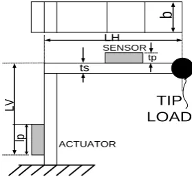
The schematic diagram of the proposed structure (i.e. inverted L) is shown in the fig 1. The structure is mounted with two piezoelectric patches bonded on its surface acting as sensors and actuators. One of which are used as actuator and the other one as a sensor. The geometrical and mechanical properties of the structure are listed in table I. The Lagrange’s equations of motion for linear systems are given as below

( )

( )

( )

m t c k t

n _{ji i ji i ji i}

t i,j 1,2,...,n

i 1 _j

⎡ _{Δ + Δ + Δ} ⎤

⎢ ⎥

⎣ ⎦

∑

= =

=

Q

(1)

where Δ(t), Δ. (t) and (t)Δ.. are the physical displacement, velocity and acceleration respectively. Fig.1 shows the geometry and boundary conditions of the structural system. The eigenvalue problem can be solved to give the natural frequencies and mode shapes for various tip loads ranging from 0g – 20g. These modal parameters can be used to construct the system matrices [9, 10].

b

tp ts

lp _ACTUATOR

SENSOR

TIP LOAD

LH

LV

Fig.1: Schematic diagram of the inverted L structure

Table I: Geometrical and mechanical properties of the structure

Material

Property Steel PZT

Length of Horizontal limb(mm) LH= 100 ---

Length of Vertical Limb(mm) LV=100 ---

Thickness(mm) ts=1 tp=1

Length(mm) --- lp=20

Width(mm) B=10 b=10

Young’s Modulus(Mpa) Es=210 Ep=64

Density(Kg/m3_{) ρ}

s =7800 ρp=5670

Distance of sensor from Free end i.e. x (mm)

60

Distance of actuator from Fixed end i.e. y (mm)

20

Distance of primary source of disturbance from jointed point

i.e. z (mm)

20

B. Piezoelectric Sensing and Actuation

When bending moment is given to the structure mounted with PZT patch, certain electrical charge is developed in the patch [11]. Certain voltage is developed by this charge. This developed voltage is a function of the strain developed in the flexible structure on which this PZT patch is attached. On the other hand if a voltage V is applied to a patch attached on a distributed structure, a bending moment is produced [12]. This bending moment is used to reduce the vibrations.

III. ADAPTIVE POLE PLACEMENT FEEDBACK CONTROLLERS

In transfer function form, the structural system can be represented as a ratio of two polynomials G=B/A. An output feedback is applied to the system which has a transfer function given by H=G/F. The overall transfer function of the system is given by

1

= = =

+ +

P G BF

T

Q GH AF BG (2)

which has CL zeros in P and CL poles in Q. The co-efficient of the polynomial equation Q

IV ROBUST POLE PLACEMENT CONTROL

It is well known that in order to design a robust controller the choice of CL poles depends critically on plant transfer function. An arbitrary choice of stable CL poles can lead to a very poor controller design for certain plants. The present approach seeks to find controllers which minimize (in some sense) the sensitivity of CL poles to perturbations in plant or system parameters. In the present work, only Single-Input, Single-Output case is analyzed and implemented.

Let q=[q0 q1 …….q2n-1 ] be the polynomial co-efficient of Q(z-1). Defining v =[a0 a1 ….. an b0 b1 ….bn] as the system vector, x =[h0 h1 ….hn-1 g0 g1 …..gn-1] as the controller vector and θ as a 2n x (2n+2) matrix of shifted controller parameters (Sylvester form) i.e.

0 0

1 1

n -1 0 n -1 0

n -1 0 n -1 0

n -1 n -1

h 0 0 g 0 0

h g

= h h 0 g g 0

0 h h 0 g g

0 h 0 g

θ

⎡ ⎤

⎢ ⎥

⎢ ⎥

⎢ ⎥

⎢ ⎥

⎢ ⎥

⎢ ⎥

⎢ ⎥

⎢ ⎥

⎢ ⎥

⎣ ⎦

… …

… …

(3)

Then it is very straight forward to write the CL pole placement equation as θ v =q. The pole placement problem becomes that of determining the controller vector x (whose components are in θ) such that θ v =q. When the system vector v is uncertain (i.e. assumed to lie in a range), the controller x obtained from the above equation may not be able to stabilize the CL system for perturbations of v from its nominal value [17].

In order to develop a robust solution, it will initially assumed that a s and b s have independent interval coefficients; hence the system vector v becomes an interval vector [v- , v+]. If we assume that there is certain flexibility in desired pole locations so that q becomes an interval vector [q- , q+]. The controller can be designed by choosing the nominal system vector

v0, a nominal desired pole vector q0, system error

vector μ and a pole assignment flexibility error vector ε as follows [17]

- 0 + 0

- 0 + 0

v =v -μ and v =v +μ

q =q -ε and q =q +ε (4)

Then the set of all robust pole placement controllers is given by

{

}

S x:θ(x) v - q ≤ ∀ε v: v-v ≤μ (5) where the mod operation is taken to be component wise. To find a time invariant robust controller in S that will take every system vector _{v [v , v ]}∈ - + _{and map into any}

CL system vector _{q [q ,q ]}∈ - + _{can be posed as}

robust pole placement problem as

0 2n

0 0

minimize f(x)= - ; x

subjected to θ(x) v - q ε v: v-v μ

∈

≤ ∀ ≤

x x

(6)

where x0

can be any desired controller. x0 can

be found by solving the pole-placement problem for the nominal system and nominal desired pole positions. i.e. θ0 _v0 _=q0_{. The}

robust pole-placement seeks to find controller vector x* which guarantees that the CL polynomial coefficients q remain within the prescribed regions for all prescribed uncertainties in the system vector v. In order to present the above optimization problem into more tractable mathematical optimization form, the following results are needed.

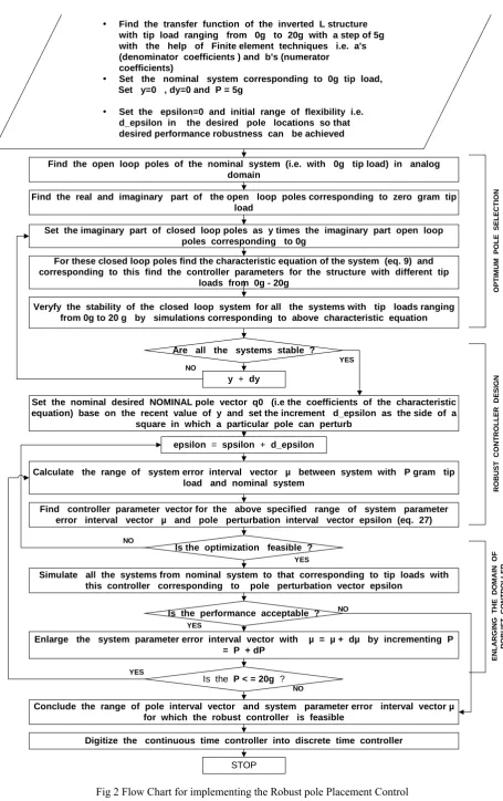
y Find the transfer function of the inverted L structure with tip load ranging from 0g to 20g with a step of 5g with the help of Finite element techniques i.e. a's (denominator coefficients ) and b's (numerator

coefficients)

y Set the nominal system corresponding to 0g tip load, Set y=0 , dy=0 and P = 5g

y Set the epsilon=0 and initial range of flexibility i.e. d_epsilon in the desired pole locations so that desired performance robustness can be achieved

Find the open loop poles of the nominal system (i.e. with 0g tip load) in analog domain

Find the real and imaginary part of the open loop poles corresponding to zero gram tip load

Veryfy the stability of the closed loop system for all the systems with tip loads ranging from 0g to 20 g by simulations corresponding to above characteristic equation

y + dy

Find controller parameter vector for the above specified range of system parameter error interval vector µ and pole perturbation interval vector epsilon (eq. 27)

Are all the systems stable ?

For these closed loop poles find the characteristic equation of the system (eq. 9) and corresponding to this find the controller parameters for the structure with different tip

loads from 0g - 20g

Set the imaginary part of closed loop poles as y times the imaginary part open loop poles corresponding to 0g

Calculate the range of system error interval vector µ between system with P gram tip load and nominal system

Is the optimization feasible ?

Set the nominal desired NOMINAL pole vector q0 (i.e the coefficients of the characteristic equation) base on the recent value of y and set the increment d_epsilon as the side of a

square in which a particular pole can perturb

epsilon = spsilon + d_epsilon

Enlarge the system parameter error interval vector with µ = µ + dµ by incrementing P = P + dP

Is the performance acceptable ?

STOP

Simulate all the systems from nominal system to that corresponding to tip loads with this controller corresponding to pole perturbation vector epsilon

Conclude the range of pole interval vector and system parameter error interval vector µ for which the robust controller is feasible

YES NO

YES NO

YES

NO

Digitize the continuous time controller into discrete time controller

O

P

T

IM

U

M

PO

L

E

SEL

ECT

IO

N

R

O

BU

S

T

CON

T

ROL

L

E

R

DE

S

IGN

ENLAR

G

ING

TH

E

DO

M

A

IN O

F

RO

BU

ST

C

O

N

T

RO

L

L

E

R

Is the P < = 20g ?

YES

NO

V. IMPLEMENTATION AND VERIFICATION OF CONTROL SYSTEMS

A. Experimental Setup and Procedure

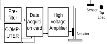
The schematic view of the inverted L structure along with the hardware is shown in the fig 3. The inverted L structure is equipped with 2 PZT patches. To bear the computational burden LABVIEW based real time engine 8187 RT is used.

COMP-UTER

Data Acquiti-on card

High voltage Amplifier

Actuator Sensor

Pre-filter

Tip Load

Fig 3 Schematic diagram of the experimental setup

B. Simulations and Experimental Results

First the nominal system is taken pertaining to 0g tip load. CL system poles are fixed taking the system parameters into account. The controller is then designed by solving the Diophantine equation. The tip load is changed from 0g to 15g for the first structure and 0g to 60g for second structure. Maximum available actuator voltage is taken as the 220 volt.

C. Performance of Adaptive Pole Placement Controller

First of all numerical simulations are carried out to understand the dynamics of the CL system with adaptive pole placement controller (APPC) and robust pole placement controller (RPPC) afterwards experimental implementation was done. Part (a) of fig. (4) Shows the response of the adaptive control system for structure-I with zero gram tip load. The OL and CL response is almost the same i.e. no control effectiveness. This is in contrast to the response of the same structural system if non-adaptive controller is applied. This means that any arbitrary pole locations of the CL poles, system gives severely deteriorated performance of adaptive control system for the nominal system (i.e. at 0g tip load). But, if the imaginary part of the CL pole locations is made smaller, performance improves.

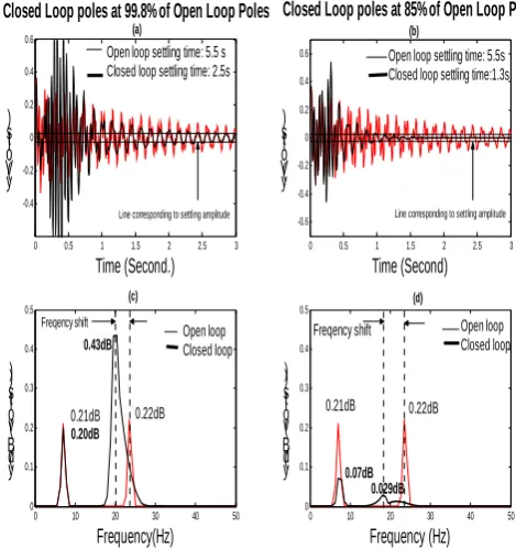
The optimal performance is obtained when the CL pole is 0.85 times the imaginary part of the OL pole locations (i.e. with a large movement of the pole position towards origin on vertical axis); this defect was clearly eliminated (fig 4b). Similar deterioration in performance was observed if the tip load was changed from 0g to 15g (fig 5a). The transition response is not so good. The amplitude of the CL system increases as compared to OL system during initial time steps. Also the CL settling time is large (i.e. 2.5 second ) as compared with the second case ( with CL settling time of 1.3 second) where the imaginary part of the CL pole locations are made 0.85 times the imaginary part of the OL pole locations (fig 5b). Obviously, higher control voltages will be needed in the later case. By constraining the control voltage to a certain magnitude which is available practically, this problem can be solved. By observing the response in frequency domain (fig 5c), it is observed that, although the first mode amplitude is reduced, the second mode gets excited. However, by using optimal location of CL poles, better performance gets resulted (fig 5d).

0 0.5 1 1.5 2

-0.5 0 0.5

y(V olt s)

CL poles at 99.8% of OL Poles

0 0.5 1 1.5 2

-150 -100 -50 0 50 100 150

u(V olt s)

0 0.5 1 1.5 2

-0.5 0 0.5

y(V olt s)

Time (Second)

0 0.5 1 1.5 2

-150 -100 -50 0 50 100 150

Time (Second) u(V

olt s)

CL poles at 85% of OL Poles

(a) (b)

(c) (d)

OL response CL response

OL response CL response

Fig 4 Effect of different positions of closed loop poles on the performance of adaptive controller for nominal

0 0.5 1 1.5 2 2.5 3 -0.4 -0.2 0 0.2 0.4 0.6 y (V olt s ) Time (Second.)

0 10 20 30 40 50

0 0.1 0.2 0.3 0.4 0.5 y(d B(v olt s)) Frequency (Hz)

0 0.5 1 1.5 2 2.5 3 -0.6 -0.4 -0.2 0 0.2 0.4 0.6 y (V olt s ) Time (Second)

0 10 20 30 40 50

0 0.1 0.2 0.3 0.4 0.5 y(d B(v olt s)) Frequency(Hz)

Open loop settling time: 5.5s Closed loop settling time:1.3s Open loop settling time: 5.5 s

Closed loop settling time: 2.5s

Open loop Closed loop

Open loop Closed loop

(a) (b)

(c) (d)

Line corresponding to settling amplitude Line corresponding to settling amplitude Closed Loop poles at 99.8% of Open Loop Poles Closed Loop poles at 85% of Open Loop Poles

0.21dB 0.20dB

0.22dB

0.43dB Freqency shift Freqency shift

0.21dB 0.22dB

0.07dB 0.029dB

Fig 5 Effect of different positions of closed loop poles on the performance of adaptive controller at 15g tip load

D. Performance of Robust Pole Placement Controller

Table II shows the limiting amplitude of the actuator voltages for both the structures at different tip loads for adaptive pole placement controller (APPC) and robust pole placement controller (RPPC). For both the structures APPC requires high voltage for stable operations.

TABLE II Performance comparison of adaptive and robust pole placement control Maximum Actuator Voltage (volts) required No. of the struc ture Ori gin al Wei ght (O W) Tip Load OW/B M APPC RPPC

0g 578 --- ---

5g 867 150 30 10g 1156 180 60 15g 1441 220 100

Struc ture I

10.5 g

20g --- UNSTAB

LE UNSTABLE

0g 1127 -- --

14g 1433 190 30 30g 1741 640 25

Struc ture II

57.3 g

60g 2356 130 30

E. Performance Comparison of Adaptive and Robust Pole Placement Controller

The structure was excited by a constant velocity excitation. A steel ball was thrown from a certain height near the tip or at the mid of the horizontal limb. A certain auto-regressive model of order 12 was used to model the measurement noise. Excellent CL results were obtained (fig 6). So, if the noise can be modeled properly, RPPC is the best choice for both light weight as well as heavy structures.

0 0.5 1 1.5 2 2.5 3 3.5 4

-0.5 0 0.5 y(v olt s) Time(second)

0 0.5 1 1.5 2 2.5 3 3.5 4

-150 -100 -50 0 50 100 150 u(v olt s) Time(sec) Open Loop Closed Loop

Fig 6 Performance of robust controller at 15g tip load WITH modeling the measurement noise (Experimental)

VI CONCLUSION

REFERENCES

[1]. Zeng Y, Araujo and Singh SN, “Output feedback variable structure adaptive control of a flexible spacecraft,” Astronautica, 44(1), 1999, pp. 11-22

[2]. Youn SH, Han JH and Lee I, “Neuro-adaptive vibration control of composite beams subjected to sudden de-lamination,” Journal of sound and vibration, 238(2), 2000, pp. 215-231

[3]. Shaw J, “Adaptive control for sound and vibration: A comparative study, ” Journal of sound and vibration,

235(4), 2000, pp. 671-684

[4]. Rew KH, “Multi-modal vibration control using adaptive positive position feedback,” Journal of intelligent materials and structures, 13 (1), 2002, pp.

13-22

[5]. Bai MR, “Experimental evaluation of adaptive predictive control for rotor vibration suppression,”

IEEE transactions on control system technology,

10(6), 2002, pp. 895-901

[6]. Lim CW, Chung TY and Moon SJ, “Adaptive bang-bang control for the vibration control of structures under earthquakes,” Earthquake Engineering and Structural Dynamics, 32(13), 2003, pp. 1977-1994

[7]. Lee YS and Eillot SJ, “Active Position Control of a Flexible Smart Beam using Internal Model Control,”

Journal of Sound and Vibration, 242(5), 2001, pp.

767-791

[8]. Crassidis JL, Amr Baz and Norman Wereley, “H infinity control of active constrained layer damping,”

Journal of vibration and control, 6, 2000, pp.

113-136

[9]. Liu TX, Hua HX and Zhang Z, “Robust control of plate vibrations via active constrained layer damping,” Thin Walled Structures, 42, 2004, pp.

427-448

[10]. Xie SL, Zhang XN and Zhang JH, “H infinity Robust vibration control of a thin plate covered with a controllable constrained damping layer,”

Journal of vibration and control, 10, 2004, pp.

115-133

[11]. Rogelio Lozano and Xiao Hui Zhao, “Adaptive pole placement without excitation probing signals,” IEEE Transactions on Automatic Control, 39(1), 1994, pp. 47-58

[12]. Meirovitch, “Elements of Vibration Analysis,”

McGraw Hill Publishing Company, New York, 1986

[13]. Meirovitch, “Dynamics and Control of Structures” John Wiley and sons, UK, 1986

[14]. Buttler R and Vittal Rao, “A State Space Modeling and Control Method for multivariable smart structural Systems,” Smart Materials and Structures, 5, 1996, pp. 386-399

[15]. Baz A, and Poh S, “Performance of Active Control System with piezoelectric actuators,”

Journal of Sound and Vibration, 126(2), 1988,

pp. 327-343

[16]. Wellstead PE, D Prager and P Zanker, “Pole Assignment self tuning regulator,” Proc. IEE Control Science, 126, 1979, pp. 781-87.

[17]. Soh YC, Evans RJ Petersen IR and Betz RE, “Robust Pole Assignment,” Automatica, 23 (5),

1987, pp. 601-610

[18]. Barmish BR, “Invariance of strict Hutwitz property for polynomials with perturbed coefficients,” IEEE Transactions on Automatic Control, 29 (10), 1984, pp. 935-936

[19]. Brain L Stevens and Frank L Lewis, “Aircraft control and simulations,” John Wiley and Sons,

New Jersey, 2003

[20]. Routh EJ, “Stability of motion,” Taylor and