A Statistical Decision Making Method: A Case Study on Prepositional Phrase Attachment

(1)

A Statistical Decision Making Method: A Case S t u d y on

Prepositional Phrase Attachment*

M e h m e t Kayaalp, Ted P e d e r s e n and R e b e c c a B r u c e

Department of Computer Science & Engineering

Southern Methodist University

Dallas, TX 75275-0122

{kayaalp, pedersen, rbruce}@seas, smu.

edu

A b s t r a c t

Statistical classification methods usually rely on a single best model to make accurate predictions. Such a model aims to maximize accuracy by balancing precision and recall. The Model Switching method as presented in this paper performs with higher predictive accuracy and 100% recall by using a set of decomposable models instead of a single one.

The implemented system, MS1, is tested on a case study, predicting Prepositional Phrase Attachment (PPA). The results show that iV is more accurate than other statistical techniques that select single models for classification and competitive with other successful NLP approaches in PPA disambiguation. The Model Switch- ing method may be preferable to other methods because of its generality (i.e., wide range of applicability), and its competitive accuracy in prediction. It may also be used as an analytical tool to investigate the nature of the domain and the characteristics of the data with the help of generated models.

1 I n t r o d u c t i o n

Decision problems are classically defined as problems whose answers fall in either of two classes: Yes and No (Garey and Johnson, 1979). Optimization problems are another class of problems that maximize or minimize some value; however, they can be cast as decision problems as well (Cormen et al., 1990). Classification problems incorporate the characteristics of both: A classification problem is a decision

*This research was supported in part by the Office of Naval Research under grant number N00014-95-1-0776

problem, in which a decision is made (a class is selected) that maximizes a utility function (yon Neu- mann and Morgenstern, 1953). The Model Switch- ing method as proposed in this paper can be used with any utility function (decision criterion) for any decision problem with categorical data that can be represented as a tuple (C, F1, F2, ..., Fn) of a class variable C and some feature variables F{1 .... }.

In the following sections, we will describe the Prepositional Phrase Attachment (PPA) problem and various approaches to solving it. After dis- cussing the statistical concepts used in this work, we will introduce the concept of Model Switching, why it is needed, how it works, and our experience on the PPA problem with Model Switching. Comparisons with earlier works on corpus-based PPA prediction and conclusions will follow.

2 P P A P r o b l e m

Resolving the PPA problem is a common problem in any NLP system that deals with syntactic parsing or text understanding. The Naive Bayes classifier and leading machine learning systems, such as C4.5 (Quinlan, 1993), CN2 (Clark and Niblett, 1989) and PEBLS (Cost and Sahberg, 1993), fail to provide prediction with competitive accuracy rates on this problem (see Table 4 on page 40). A sentence can be so ambiguous that it may not be possible to determine the correct attachment without extra contextual information. (Ratnaparkhi et al., 1994) reported that human experts could reach an accuracy of 93%, if cases were given as whole sentences out of context.

The PPA problem is illustrated by the following example:

I described the problem on the paper. (1)

This is an ambiguous sentence, which can be interpreted two different ways, depending on the site of PPA. The prepositional phrase (PP) in the above sentence is "on the paper." If it is attached to

Kayaalp, Pedersen ~ Bruce 33 Statistical P P Attachment

(2)

the (object) noun "problem," then the interpretation would be equal to (2); on the other hand, if it is attached to the verb "describe," then it would be interpreted as (3).

I described the problem that was on the paper(2) On the paper, I described the problem. (3)

In this paper, we address only the type of PPA problem illustrated above and don't consider other less frequent PPA problems. For the linguistic details of the problem, the reader can refer to (Hirst, 1987).

We use the PPA d a t a created by (Brill and Resnik, 1994) and (Ratnaparkhi et al., 1994) to objectively compare the performances of the systems. Both d a t a were extracted from the Penn Treebank Wall Street Journal (WSJ) Corpus (Marcus et al., 1993). In order to distinguish these d a t a from each other, we call the former one BSzR d a t a and the latter one IBM data. Both PPA d a t a were formatted in tuples with five variables (4), which denote the class (i.e., the PPA attachment site) and the features (i.e., verb, object noun, preposition and PP noun) in the respective order• Values of these variables for the above example (1) are illustrated in (5), where

(A, B, C, D, E) (4)

(verb lnoun , "describe", "problem", "on", "paper"X5)

For representation convenience, we can map the values of these variables to positive integers as in Ta- ble 1. Then, the examples, (2) and (3) can be con-

[ L e v e l s I[ A [ B ] C [ D [ E ] n o u n d e s c r i b e

v e r b j o i n b e

i m p r o v e s h i p p i n g

d e v £ 1 o p s 1

2 3

8 1 8 2

3 8 4 5 3 8 4 6

5 1 6 2 5 1 6 3

66"25

p r o b l e m o n p a p e r b o a r d a s d i r e c t o r

d e a n o f N . V .

H a t c h p l u s e n d s u c c e s s t h e y

c h u n k s s h o t s K o c h b a r

:

o p t i o n p o t ( A t i c o r p

r e b a t e

Table 1: Substitution of variable values for associated integer labels at the Levels column. The number of levels of five variables are 2, 3845, 5162, 81 and 6625.

verted to tuples (6) and (7), respectively.

( A = I , B = I , C = I , D = I , E = I ) (6) ( A = 2 , B = I , C = I , D = I , E = I ) (7)

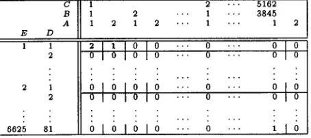
Using this convention, the PPA d a t a can be represented in a contingency table (Table 2) with five dimensions, where each dimension is dedicated to a variable. The size of a contingency table is determined by the cardinality of values (a.k.a. levels) of these variables (8); for the IBM data, there are 2.13 × 1013 cells in the table (9). Each cell in the table corresponds to a unique combination of the variable values and all combinations are represented in the table.

C B A E D

I I 2

2 i

2 1 1 2 1 2 1 2

L,1010

0 0 0 0

0]01010

2 . . . 5 1 6 2 . . . 1 . - . 3 8 4 5 • . . 1 . . . 1 2

• ' ' 0 . . .

• . • 0 . . •

. - - 0 . . . 1 ] 0 I 0 [ 0 0 0

0[0

Table 2: The PPA d a t a can be represented in a 2 × 3845 x 5162 x 81 × 6625 contingency table, where each cell contains frequency with which the corresponding 5-tuple (i.e., a unique PPA instance) occurs in the data.

(IAI =2, ]BI =3845, ICI =5162, IDI--81, IEI =6625)(8) 2 × 3845 × 5162 × 81 × 6625 = 2.13 x 1013 (9)

Considering t h a t there are 27,937 PPA observations in the training and test d a t a together, a search space of more than 21 trillion possible distinct cases (represented in the cells of contingency table) indicates t h a t the d a t a is extremely sparse.

To solve PPA problem, NLP researchers designed domain specific classifier systems. Those systems can be categorized in two classes:

1. Rule based systems (Boggess et al., 1991), (Brill and Resnik, 1994)

2. Statistical and information theoretic approaches (Hindle and Rooth, 1993), (Ratna- parkhi et al., 1994),(Collins and Brooks, 1995), (Franz, 1996)

[image:2.596.316.543.233.334.2] [image:2.596.76.294.481.643.2]

(3)

and preposition, respectively. While (Hindle and Rooth, 1993) stated t h a t this approach was not successful in estimating PPA using small 2-tuple fre- quencies, which comprised a major portion of the PPA data, the accuracy reported was 79.7%, which is a substantial improvement over the lower bound of 65% (10):

tions used in the function). If all fail, the assign- ment is noun attachment, since 52% of the time the attachment site on the training d a t a was noun.

I~(A]B, C, D, E) =

I ( A , B , C , D ) + I ( A , B , D , E ) + ] ( A , C , D , E ) ](B, C, D) + I(B, D, E) + ](C, D, E) (12)

f(A = 1) f ( A = 2) "1 max

f(A=~)+~=2)' f(A--'~)~-?~--2)

(10)

The lower bound for the B&R d a t a is 63% (Brill and Resnik, 1994) and for the IBM d a t a is 52% (Ratna- parkhi et al., 1994).

(Ratnaparkhi et al., 1994) was the first to considered the full four feature set defined in (4). The approach made use of a maximum entropy model (Berger et al., 1996) formulated from frequency information for various combinations of the observed features. The combinations that reduced the entropy most, were chosen. The accuracy of PPA classification using this approach was 77.7% on the IBM data. (For performance comparison of various approaches on available data, please refer to Table 4 on page 40.)

(Brill and Resnik, 1994) suggested a rule based approach where the antecedent of each rule specifies values for the feature variables in (4). A typical rule might be as follows:

f e a t u r e s ( B = 12, C, D = 3, E) -+ ppa(A = 1) (11)

471 such inference rules are found useful and ordered to reduce the error-rate to a minimum. They reported an accuracy of 80.8% on the d a t a t h a t we also use. They also duplicated the experiment of (Hindle and Rooth, 1993), which scored around 5% less than the rule-based approach.

(Collins and Brooks, 1995) proposed a specific heuristic computation to predict PPAs. The idea originated from the back-off model (Katz, 1987). If the combination of feature values observed for a test instance is also observed in the training set, then t h a t test instance is classified with the most frequent PPA site for those feature values in the training set. Otherwise, probability estimates for the two PPA sites are obtained from functions(12)-(14), via a process similar to model switching. If the highest complexity formulation, (12), cannot be used to classify a test instance (i.e., the required feature value combinations are not observed in the training data), then the decision process is switched to the next function, where functions are ranked based on complexity (i.e., the arity of the frequency distribu-

f f ( A ] B , C , D , E ) = ] ( A , B , D ) T I ( A , C , D ) T J ( A , D , E ) f l 3 ~ I ( B , D ) + f ( O , D ) + f ( D , E) " " I~(AID) -- ] ( A , D ) (14)

f ( D )

If a higher order function cannot classify a test instance, then the decision process is switched to the next function. If all fail, the guess is the noun attachment, since 52% of the time the attachment site on the training d a t a was noun.

While the probability estimates in (14) are maxi- m u m likelihood estimates (MLEs), the estimates in (12) and (13) are heuristic formulations (i.e., not MLEs). The rationale behind these formulae are:

1. a decision made by utilizing more feature variables should be favorable over the others,

2. the preposition feature D is essential; thus, it is better to keep it in all n-grams of the decision functions.

They used IBM data, which we also use, and reported an accuracy of 84.1%.

(Franz, 1996) proposed a new feature set, which provided a more compact representation of the PPA data. Using a hierarchical log-linear model con- taining only second order interactions, he achieved a classification performance comparable to t h a t of (Hindle and Rooth, 1993). He also designed another experiment with a less common PPA problem with three attachment sites.

3 D e c o m p o s a b l e M o d e l s

In this paper, PPA is cast as a problem in supervised learning, where a probabilistic classifier is induced from tagged training d a t a in the form of 5-tuples (6) and (7). The task is to predict the value of the tag A given the values of the feature variables B through E.

(4)

test d a t a instance represented by a 4-tuple of feature values.

Decomposable models belong to the class of graph- ical models, 1 where variables are either interdepen- dent or conditionally independent of one another. 2 All graphical models have a graphical representation such t h a t each variable in the model is mapped to a vertex in the graph, and there is an undirected edge between each pair of vertices corresponding to a pair of interdependent variables. While edges represent interactions between pairs of variables, i.e., second order interactions, cliques 3 with n vertices represent

n t h order interactions. Any two vertices t h a t are

not directly connected by an edge are conditionally independent given the values of the vertices on the path t h a t connects them.

Decomposable models are graphical models t h a t are isomorphic to chordal graphs. In chordal graphs, there is no cycle of four or more without a chord, where a cord is an edge joining two non-consecutive vertices on the cycle. T h e elementary components of a chordal graph are its cliques; therefore, a chordal graph can be represented as a set of its cliques.

T h e chordM graph in Figure 1 represents a decom-

E

B

A

Figure 1: T h e decomposable model

A B D . A B E . A C E . Edges of the separators, A B and A E (corresponding to A B D N A B E and A B E N A C E ) , are drawn thicker. A separator is a set of vertices whose removal disconnects the graph.

posable model, which we can mnemonically denote as (15).

A B D . A B E . A C E (15)

In this model, variables A, B, and D are stochas- tically dependent since they form a clique. Simi- lar statements can be made for the other cliques in the model. T h e interactions between A B and AE,

1 Graphical models are a subset of log-linear models. 2B and C are conditionally independent given A if P(BIC, A ) = P(BIA ).

3A clique is a complete (sub)graph, where every vertex pair is connected with an edge.

denoted by the corresponding edges A B , A E are observed in two out of the three cliques which indicates their relative importance in describing this distribution. T h e variable A is observed in all three cliques of the model because we consider only those cliques t h a t contain the class variable A in defining the model. There are three edges missing, BC, CD, and DE, which distinguish this model from the saturated model A B C D E . These missing edges denote three conditional independence relations:

1. The variables D and E are conditionally independent given A B (intersection of two cliques, A B D N A B E ) .

2. T h e variables B and C are conditionally independent given A E ( A B E n A C E ) .

3. The variables C and D are conditionally independent given A ( A B D N A C E ) .

This approach to classifying PPA is the first to make use of conditional independence in modeling the distribution of feature variables.

A well known example of a decomposable model is the Naive Bayes model in which all feature variables are conditionally independent given the value of classification variable. For the PPA problem, the Naive Bayes model is A B . A C . A D . A E .

Decomposable models are i m p o r t a n t because they are those graphical models t h a t express the joint probability distributions of the variables in terms of the product of their marginal distributions, where each factor of the product corresponds to a clique or a separator in the graphical representation of the model. Because the joint distribution functions of decomposable models have such closed-form expres- sions, the parameters as Maximum Likelihood Esti- mates (MLEs) can be calculated directly from the training d a t a without the need for an iterative fit- ting procedure; hence, those MLEs are also called direct estimates (Bishop et al., i975).

3.1 M a x i m u m L i k e l i h o o d E s t i m a t i o n

Let the PPA variables, IAI = I, IBI = J , . . . , IEI = M resulting in an I × J x K x L x M contingency table (e.g., Table 2). Let the count in each cell (i.e., the frequency with which the corresponding 5-tuple is observed in the training data) be denotes as nijktrn. When all variables are considered to be interdependent (i.e., the saturated decomposable model) the m a x i m u m likelihood estimate of the probability of any 5-tuple is equal to the count in the corresponding cell noklm divided by the total count N, which is equal to 24,840 for the IBM training d a t a (Table 2).

(5)

911111 - - r t l l l l l 2

N - 24840 (16)

Estimates of the marginal probability distributions can be calculated in a similar fashion. If we are interested in the probability of observing a verb a t t a c h m e n t when "describe" is the noun, and "on" is the preposition (i.e., A = 1 , B = 1, D = 1), re- gardless of the values of the other variables, it can be calculated as in (17) and (18).

K M

n i l + i + = E E nnkl,~ (17) k = l m = l

n n + l + (18)

9(A=I,B=i,D=I)

= p l l + l + - N

Let c denote the specific cell coordinates (e.g., 11111 in (16)), and let the model .A4 = {C: U C2 U

• . . C O }, where Cd denotes a clique in the graph rep-

resentation of A//, then the direct estimates (MLEs) are computed as in (19).

D ^

~n(c) Hd=l

p(cc,,)

- - D ^

Hd=2

p(es )

(19)

where the factors in the numerator are the marginal probabilities for c in the cliques

{Cd},

whose union represents the model. The intersections of cliques

{Cd}

yield separators {Sa} and the marginal prob-

abilities for c in

{Sd}

are factors in the denomi- nator (Lauritzen, 1996). For the saturated model, {,.~} = {}, and the MLE is most straightforward:

= 9c (20)

m l l l n = 911111 (21)

MLEs of the model (15) can be computed as in (22), and using this model, MLEs of the examples (2) and (3) can be calculated as in (23) and (24), respectively.

=

~ 2 t l : l l I =

m21111

9(A, B, D) 9(A, B, E) 9(A, C, E t 2 2 ) 9(A, B) 9(A, E)

91:+1+ 9 n + + l P : + l + l (23)

9 1 1 + + + 9 1 + + + 1

921+I+ 921++1 P2+i+i

(24)

92i+++ 92+++l

As seen in this example, decomposable models provide us not only a very powerful representation medium but also computational efficiency in estimating parameters.

4

Model Switching

Let E1 and E2 be equal to MLEs in (23) and (24). There are four cases in determining the class based on these equations.

E i = 0 A E 2 = 0 -4 A = n u l l (25)

El > 0 A E i = E 2 -4 A = n u l l (26)

El > $2 -+ A = 1 (27)

E1 < E2 "-')" A = 2 (28)

In cases (25) and (26), there is no classification and no recall for this test instance with this model. In (27) and (28), the classifications are noun and verb attachments, respectively.

For the PPA d a t a with five variables, there are only 110 decomposable models, corresponding to all chordal graphs of order five or less, where every clique of the order two and higher contains the vertex t h a t represents the class variable. Since this number is not large, we considered all of these models for classification. 4 Let all test instances be composed in the set T and let

T = % u % u . . . u T ~

(29)

where 7~ is a set of test instances t h a t

can

be classified with model A,4i for (1 < i < m = 110); i.e., the outcomes of ¢n(AI7~, .h4~) is either in (27) or in (28). These estimates m a y not always be correct, un- less the information in features are sufficient and the classification model is perfect; therefore, each set of estimates associated with ~ and A//i has a precision value:

precision(M lT)

- I cl

T = T c u T w

(30)

(31)

where 7~c and "/~w are sets of correctly and wrongly classified test instances in set 7~. If we have an ordered list of models (.A41, A 4 2 , . . . , .A4m) as a certificate, where

precision(.MilT~ ) > precision(A4~+: l'/~+l)

(32)

we could use the certificate to maximize the overall classification accuracy.

Since the first model .N'/1 is associated with the highest precision value, the probability t h a t a test instance is correctly classified with .A41 is higher than

(6)

t h a t probability for any other model; therefore, .M1 should be used to classify all possible test instances.

T = 7 -0 = "]~ t.9 7 -1 , where ~ VI T 1 = {} (33)

After ~ is classified, the process is repeated for the remaining test instances 7 -1 with M 2 t h a t is the m o s t "precise" model remaining in the model set. This cycle can be generalized as

7-/- 1 = 7~ t3 7 -i, where "/~ N 7 --/= { }, and T = T O (34) and will be iterated k times, where T k = {}. T h e overall classification accuracy then be calculated as

k

accuracy(.A41,.M2,.. . M k l T - ) - i=1 (35)

'

17-1

T h e question remains now, how we can find the list of models (.M1, . M 2 , . . . , . M k , . . . , .Mm) ordered by precision. Since precision is a measure t h a t can be acquired after classifying all test instances, how can we order models based on precision before testing?

One approach is to use the error rates of the models acquired t h r o u g h cross-validation. T h e technique we use here is called leave-one-out cross-validation (Lachenbruch and Mickey, 1968). Let the training d a t a set be TO, where every d a t a instance Pi E T~, i = 1 , 2 , . . . , r and r = I ~ I. W h e n a m o d e l A / / j is applied to a d a t a instance Pi, in this technique, all training instances except Pi (i.e., T¢ - pi) are used to c o m p u t e the direct e s t i m a t e for pi. This process is repeated for every d a t a instance (i.e., r times). This technique is applied to all training instances for every model. T h e precision score of each model is collected, and based on those scores, the models are ordered.

If k (the n u m b e r of models used to classify all P P A instances) is small, then it is expected t h a t after each iteration the test instances remaining to be classified would be decreased significantly; hence, the characteristics of T i-1 and T i might differ sub- stantially and ordering the remaining models based on T i, rather t h a n "T 0, m i g h t increase the overall accuracy.

A second experiment is designed to apply this recursive s t r a t e g y to order the models via the same cross-validation process. First, the m o s t precise model for the entire (training) d a t a is identified. Then, the d a t a instances t h a t are classified with the first model are excluded f r o m the original d a t a set, as in (33). Within the remaining d a t a instances, all models in {.A42, M 3 , . . . , Adrn} are searched for the current m o s t precise model. This model selection

Models [[ Cor Inc Prc Acc RTC

A B C D E A B D E . A C D A C D E . A B D

A B D E A C D E . A B E

A B C D A B D . A C D . A D E

A C D E A B D . A C D A B E . A C D . A C E

A B D A C D A B E . A C E . A D E

A C E . A D E . A B A D E

A D A D . A E A B C . A E

A C . A D A

150 17 90 89.8 2930

145 16 90 89.9 2769

192 10 95 91.9 2567

46 11 81 90.8 2510

5 0 100 90.9 2505

293 42 87 89.6 2170

441 73 86 88.3 1656

51 11 82 88.0 1594

263 50 84 87.3 1281

3 0 100 87.4 1278

401 107 79 85.5 770

296 63 82 85.1 411

0 0 0 85.1 411

6 1 86 85.1 404

156 47 77 84.5 201

141 56 72 83.7 4

0 0 0 83.7 4

1 1 50 83.7 2

0 0 0 83.7 2

2 0 100 83.7 0

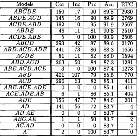
Table 3: Classification with Multiple Models. Cor (Inc): N u m b e r of correct (incorrect) classifications. Prc: Precision x l 0 0 . Acc: Accuracy x l 0 0 . RTC: Remaining Test Cases.

cycle is iterated exhaustively (34) until all d a t a instances are classified. T h e models selected for the IBM d a t a are shown in Table 3.

T h e MLE algorithm is a table look up, where each table contains m a r g i n a l values for a clique of variables as defined in the graph representation. If those values could be stored in a m e m o r y array, the t i m e complexity of M L E could be O(1); however, the n u m b e r of values is huge, thus we have to store each set of clique marginals on disk, and currently the access to the d a t a is t h r o u g h sequential file access with a t i m e complexity O(n), where n is the n u m b e r of training instances. MLEs need to be c o m p u t e d for m models and for n training instances. During each recursive step a considerable p a r t of the training instances are classified (around 5%); thus we m a y represent the process as

g = rnn ~ (36)

19

T ( N ) : T ( ~ N ) + g (37)

O ( N log N ) (38)

Therefore, the average t i m e c o m p l e x i t y for the current p r o g r a m is O ( m n 2 log(mn2)), b u t t h r o u g h memoization, 5 the overhead of the recursion will be drastically reduced in newer versions of the p r o g r a m .

[image:6.596.317.543.104.329.2]

(7)

T h e software of MS1 is developed in Perl and is freely available for research purposes only. Inter- ested parties m a y contact the first author.

5 D i s c u s s i o n

In some of the earlier works on P P A there are as- pects of the model switching framework. For example, (Brill and Resnik, 1994) ordered rules to minimize the error-rate in P P A classification. Each of these inference rules m a y be considered a decision function in a decision list. Whenever a higher order rule fails, the control switches to the next rule to classify t h a t test instance. (Collins and Brooks, 1995) ordered heuristic decision functions by complexity (arity) and classified test instances with the m o s t complex applicable function.

Non-recursive Model Switching consists of two phases:

1. Ordering available models (e.g., via leave-one- out cross-validation),

2. Applying the model on t o p of the list to the test data; whenever t h a t model does not yield any estimate, the system switches to the next model on the list.

T h e first phase corresponds to the learning phase of learning systems; whereas, the. last phase can be conceptualized as a decision list (Rivest, 1987) and (Kohavi and Benson, 1993), where the control is con- ditioned by the availability of a direct estimate given a model with a test instance. 6

In the recursive version of the Model Switching, however, the model list is d y n a m i c a l l y changed since the above phases are within a loop, where in each iteration all instances of the available d a t a are considered for classification and those which are classified are excluded f r o m the d a t a for the next iteration. T h e base case of recursion is reached when all instances are classified.

Although in this work we suggest a precision- driven model ordering scheme, the Model Switching m e t h o d enables one to use any other utility function such as accuracy or F-measure. There are other utility functions t h a t need not be acquired through cross-validation, b u t rather can be collected by an- alyzing the entire training set as in statistical significance analysis (e.g., G 2, Pearson's X2), or infor- m a t i o n criteria (e,g., Akaike or Bayes Information Criteria etc.), which can be used as well.

An advantage of this m e t h o d is t h a t we make use of a complex and powerful set of models. Much of

6This relevance of decision lists was indicated by Mike Collins in our personal discussions.

the earlier P P A research was confined to singleclique models, such as A B C D or AB, which are a small subset of decomposable models.

5.1 Q u a n t i t a t i v e A n a l y s i s

Statistical (decomposable) model selection techniques were first applied to N L P problems by (Bruce and Wiebe, 1994). Those model selection techniques aim to find a single best model b u t they alone do not perform as well as Model Switching, since even the m o s t accurate decomposable model, A B . A D , had a classification accuracy of 77%.

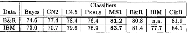
Unlike Model Switching, the m e t h o d s suggested in earlier P P A works are usually tailored to the P P A problem, thus it is hard to transfer t h e m to another domain. On the other hand, neither Naive Bayes nor the conventional machine learning tools, such as CN2, C4.5 and PEBLS, p e r f o r m as well. These four symbolic classifiers are well known and are diverse to some extent: Naive Bayes is a simple Bayesian approach, CN2 is based on rule induction, C4.5 is based on decision trees, and PEBLS is based on nearest neighbor m e t h o d . A performance comparison of various classifiers with MS1 is given on Table 4. T h e comparison between the proposed systems solving P P A a m b i g u i t y and general machine learning sys- t e m s was always neglected in earlier articles on P P A problem .7

T h e results of the first five classifiers presented in Table 4 and the performance of B & R classifier on IBM d a t a were determined as p a r t of this study, while the other four results are b e n c h m a r k s quoted from the authors cited above. Those b e n c h m a r k s were produced via single trials, hence we performed single trial tests as well. CN2, C4.5 and PEBLS performances were based on their default settings. T h e only exception involved CN2 where an ordered- induced-rule-list is used instead of an unordered one, since the ordered rules yield 99.7% accuracy ver- sus 90.8% accuracy of unordered rules on the IBM training data. After the test, we checked the accuracy rates of unordered induced rules, which are unexpectedly better t h a n the ordered ones: 78% on B ~ R d a t a and 76.2% on IBM data. Naive Bayes' recall values are very low: 74% for IBM d a t a and 78% for B & R data; therefore, the remaining test instances are classified as the m o s t frequent class. Notice t h a t this is also a t y p e of model switching, where the forms of the models and the model list M = ( A B . A C . A D . A E , A) are predetermined as done by (Collins.and Brooks, 1995).

(8)

I

Classifiers

]

Data Bayes CN2 C4.5 PEBLS M S 1 I B ~ R IBM C&B I B & R 74.6 77.4 78.4 76.4 81.2 I 80.8 n.a. 81.9 I

IBM 73.0 70.7 79.6 76.9 83.7 81.4 77.7 84.1

Table 4: Performances of various classifiers on available data. CK:B:(Collins and Brooks, 1995); B~R: (data/classifier) by (Srill and Resnik, 1994); IBM: (data/classifier) by (Ratnaparkhi et al., 1994); Bayes: Naive Bayes with defaults, i.e., A/[ = (AB.AC.AD.AE, A).

The performance differences between MS1 and C&B, the Back-off Model by (Collins and Brooks, 1995), are 0.4% for IBM data and 0.7% for B ~ R data. With only two test trials and without any deviation measure these differences cannot be considered significant, especially in this case, where the performances of the classifiers fluctuate 2-3% (e.g., C~B accuracy deviates 2.2%) within two very similar data sets, B ~ R and IBM data. As one anony- mous reviewer indicated, the 0.7% accuracy differ- ence on B&R data needs to be evaluated cautiously due to the size of the B ~ R test data, which contains only 500 test instances; whereas the IBM data contains 3097 test instances.

5.2 Qualitative

A n a l y s i s

The approach of (Collins and Brooks, 1995) is simpler than MS1, since it doesn't consist of any learning part; the models were selected and grouped by its designers and ordered heuristically, which means classification requires prior knowledge specific to the domain. With the human expertise involved, the list of models is simpler and shorter than the list found by MS1 and it is heuristically grouped and weighted (forming a kind of mixture model), which is not the case in MS1 at this point in time; nevertheless, MS1 reached to a performance level that is competitive to the other system supported with human expertise. MS1 uses neither any lexical information nor heuris- tics with respect to the PPA problem; hence, it can be adopted and applied to any other classification problem involving categorical data. MS1 is a machine learning alternative to the system developed by (Collins and Brooks, 1995), and the ordering of the models that it produces may provide insight into the data that could aid in developing a custom mixture model.

Unlike the other techniques, MS1 generates an ordered list of models where each model provides a graphical representation of the interdependencies among variables. The user can identify relevant relations and see which features play the most significant roles; thus, one can not only predict the outcome of a classification problem with high accuracy but also

gain insight into the nature of the domain and the data under investigation. For example, MS1 identified the fact that the preposition feature (variable D) is so important that all test instances (except the last four) were predicted by models that have this variable. This was one of the most important heuristic steps in formulating the approach used by (Collins and Brooks, 1995). Further analysis of the model list by linguists may yield other observations, such as, in the first 75% of the predictions, 97% of the test instances were identified using models con- taining the interaction A B D with a precision of 86%, and in the rest of the predictions this interaction was not useful. Similar model lists can be generated on various corpora and their comparisons may reveal differences in those corpora.

MS1 and the systems by (Ratnaparkhi et al., 1994) and (Brill and Resnik, 1994) consist of a training phase, where they form certain structures

(such as rules, models, etc.) that are used with the available statistics to classify test instances; therefore, these systems can be considered true learning systems. On the other hand in systems designed by (Hindle and Rooth, 1993), (Collins and Brooks, 1995), and (Franz, 1996), the forms of models were predetermined by their designers, as in the Naive Bayes approach.

5.3 Scalability

The structure of the underlying PPA data (4) casts a difficult problem to learning system. When the number of observations grows, the levels of features (except that of the preposition, which is limited by grammar) grow proportionally. This effect was first identified by (Zipf, 1935). Due to this effect the number of cells in contingency table representa- tions explodes, which corresponds to an exponential growth in the search space.

[image:8.596.153.468.102.160.2]

(9)

quirement. The Model Switching approach is scal- able in computation time and memory: While the data size grows, the leave-one-out cross-validation technique may be switched to a simpler v-fold cross- validation technique, which is "stable" and preferable for larger data size (Breiman et al., 1984). There is always, a much simpler choice: Ranking models through statistical significance analysis or through information criteria, whose cost is O(I.M I). One problem encountered in applying Model Switching to other domains is that the number of decomposable models grows exponentially with the number of possible variables. The method of (Edwards and Havr£nek, 1987) or (Madigan and Raftery, 1994) for selecting a good subset of models for the data resolves this last concern regarding scalability. Using these techniques, the Model Switch- ing method may be applied to other NLP problems with much larger size of feature variables. Model Switching method is currently being applied to word sense disambiguation which is cast with eight features. The preliminary results are very encourag- ing, and provide evidence for the robustness of the methodology.

6 . A . c k n o w l e d g m e n t s

We gratefully acknowledge the support provided for this research by the Office of Naval Research under grant number N00014-95-1-0776. We would also like to thank Mike Collins for his constructive comments.

R e f e r e n c e s

Adam L. Berger, Vincent J. Della Pietra, and Stephen A. Della Pietra. 1996. A maximum entropy approach to natural language processing. Computational Linguistics, 22(1):39-68.

Yvonee M. M. Bishop, Stephen E. Fienberg, and Paul W. Holland. 1975. Discrete Multivari- ate Analysis: Theory and Practice. The MIT Press, Cambridge, MA.

Lois Boggess, Rajeev Agarwal, and Ron Davis. 1991. Disambiguation of prepositional phrases in au- tomatically labeled technical text. In Proceed- ing of the Ninth National Conference on Arti- ficial Intelligence, pages 155-159, Cambridge, MA. AAAI, MIT Press.

Leo Breiman, Jerome H. Friedman, Richard A. O1- shen, and Charles J. Stone. 1984. Classifica- tion and Regression Trees. Wadsworth, Bel- mont, CA.

Eric Brill and Philip Resnik. 1994. A rule, based approach to prepositional phrase attachment disambiguation. In Proceedings of the Fif- teenth International Conference on Computa- tional Linguistics (COLING-9.t).

Rebecca Bruce and Janyce Wiebe. 1994. Word-sense disambiguation using decomposable models. In Proceedings of the 32nd Annual Meeting of the Association for Computational Linguistics (ACL-9~).

Peter Clark and Tim Niblett. 1989. The CN2 induction algorithm. Machine Learning, 3:261-283.

Michael Collins and James Brooks. 1995. Preposi- tional phrase attachment through a backed-off model. In Proceedings of the Third Workshop on Very Large Corpora.

Thomas H. Cormen, Charles E. Leiserson, and Ronald L. Rivest. 1990. Introduction to Al- gorithms. MIT Press, Cambridge, MA.

Scott Cost and Steven Salzberg. 1993. A weighted nearest neighbor algorithm for learning with symbolic features. Machine Learning, 10:57- 78.

David Edwards and T h o m ~ Havr£nek. 1987. A fast model selection procedure for large fami- lies of models. Journal of American Statistical Association, 82(397):205-213.

Alexander Franz. 1996. Learning PP attachment from corpus statistics. In Stefan Wermter, Ellen Riloff, and Gabriele Scheler, editors, Connectionist, Statistical, and Sym- bolic Approaches to Learning for Natural Lan- guage Processing, volume 1040 of Lecture Notes in Artificial Intelligence, pages 188-202. Springer-Verlag, New York, NY.

Michael R. Garey and David S. Johnson. 1979. Com- puters and Intractability. W. H. Freeman and Company, New York, NY.

Donald Hindle and Mats Rooth. 1993. Structural ambiguity and lexical relations. Computational Linguistics, 19(1):103-120.

Graeme Hirst. 1987. Semantic interpretation and the resolution of ambiguity. Cambridge University Press, New York, NY.

(10)

on Acoustics, Speech, and Signal Processing,

pages 400-401. IEEE.

Ron Kohavi and Scott Benson. 1993. Research on decision lists. Machine Learning, 13:131-134.

Peter A. Lachenbruch and M. Ray Mickey. 1968. Estimation of error rates in discriminant analysis. Technometrics, 10(1):1-11, February.

Steffen L. Lauritzen. 1996. Graphical Models. Ox- ford University Press, New York, NY.

David Madigan and Adrian E. Raftery. 1994. Model selection and accounting for model uncertainty in graphical models using Occam's window.

Journal of American Statistical Association,

89(428):1535-1546.

Mitchell P. Marcus, Beatrice Santorini, and Mary Ann Marcinkiewicz. 1993. Building a large annotated corpus of English: The Penn Treebank. Computational Linguistics,

19(2):313-330.

John Ross Quinlan. 1993. C~.5: Programs for Ma- chine Learning. Morgan Kaufman Publishers, San Mateo, CA.

Adwait Ratnaparkhi, Jeff Reynar, and S~dim Roukos. 1994. A maximum entropy model for prepositional phrase attachment. In Proceed- ings of Human Language Technology Work- shop, pages 250-255, Plainsboro, NJ. ARPA.

Ronald L. Rivest. 1987. Learning decision lists. Ma- chine Learning, 2:229-246.

John von Neumann and Oskar Morgenstern. 1953.

Theory of Games and Economic Behavior.

Princeton University Press, Princeton, NJ.