Optimal Incremental Parsing via Best-First Dynamic Programming
∗Kai Zhao1 James Cross1
1Graduate Center
City University of New York 365 Fifth Avenue, New York, NY 10016
{kzhao,jcross}@gc.cuny.edu
Liang Huang1,2
2Queens College
City University of New York 6530 Kissena Blvd, Queens, NY 11367
Abstract
We present the first provably optimal polyno-mial time dynamic programming (DP) algo-rithm for best-first shift-reduce parsing, which applies the DP idea of Huang and Sagae (2010) to the best-first parser of Sagae and Lavie (2006) in a non-trivial way, reducing the complexity of the latter from exponential to polynomial. We prove the correctness of our algorithm rigorously. Experiments con-firm that DP leads to a significant speedup on a probablistic best-first shift-reduce parser, and makes exact search under such a model tractable for the first time.
1 Introduction
Best-first parsing, such as A* parsing, makes con-stituent parsing efficient, especially for bottom-up CKY style parsing (Caraballo and Charniak, 1998; Klein and Manning, 2003; Pauls and Klein, 2009). Traditional CKY parsing performs cubic time exact search over an exponentially large space. Best-first parsing significantly speeds up by always preferring to explore states with higher probabilities.
In terms of incremental parsing, Sagae and Lavie (2006) is the first work to extend best-first search to shift-reduce constituent parsing. Unlike other very fast greedy parsers that produce suboptimal results, this best-first parser still guarantees optimality but requires exponential time for very long sentences in the worst case, which is intractable in practice. Because it needs to explore an exponentially large space in the worst case, a bounded priority queue becomes necessary to ensure limited parsing time.
∗
This work is mainly supported by DARPA FA8750-13-2-0041 (DEFT), a Google Faculty Research Award, and a PSC-CUNY Award. In addition, we thank Kenji Sagae and the anonymous reviewers for their constructive comments.
On the other hand, Huang and Sagae (2010) ex-plore the idea of dynamic programming, which is originated in bottom-up constituent parsing algo-rithms like Earley (1970), but in a beam-based non best-first parser. In each beam step, they enable state merging in a style similar to the dynamic pro-gramming in bottom-up constituent parsing, based on an equivalence relation defined upon feature val-ues. Although in theory they successfully reduced the underlying deductive system to polynomial time complexity, their merging method is limited in that the state merging is only between two states in the same beam step. This significantly reduces the num-ber of possible merges, because: 1) there are only a very limited number of states in the beam at the same time; 2) a lot of states in the beam with differ-ent steps cannot be merged.
We instead propose to combine the idea of dy-namic programming with the best-first search frame-work, and apply it in shift-reduce dependency pars-ing. We merge states with the same features set globally to further reduce the number of possible states in the search graph. Thus, our DP best-first al-gorithm is significantly faster than non-DP best-first parsing, and, more importantly, it has a polynomial time complexity even in the worst case.
We make the following contributions:
• theoretically, we formally prove that our DP best-first parsing reaches optimality with poly-nomial time complexity. This is the first time that exact search under such a probabilistic model becomes tractable.
• more interestingly, we reveal that our dynamic programming over shift-reduce parsing is in parallel with the bottom-up parsers, except that we have an extra order constraint given by the shift action to enforce left to right generation of
input w0. . . wn−1
axiom 0 :h0, i:0
sh `:hj, Si:c
`+ 1 :hj+ 1, S|wji:c+scsh(j, S) j < n
rex `:hj, S|s1|s0i:c
`+ 1 :hj, S|s1xs0i:c+screx(j, S|s1|s0)
rey `:hj, S|s1|s0i:c
`+ 1 :hj, S|s1ys0i:c+screy(j, S|s1|s0)
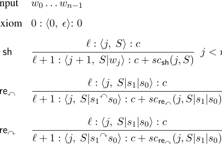
Figure 1: Deductive system of basic non-DP shift-reduce parsing. Here`is the step index (for beam search),Sis the stack,c is the score of the precedent, andsca(x)is the score of actionafrom derivationx. See Figure 2 for the DP version.
partial trees, which is analogous to Earley.
• practically, our DP best-first parser is only∼2 times slower than a pure greedy parser, but is guaranteed to reach optimality. In particular, it is ∼20 times faster than a non-DP best-first parser. With inexact search of bounded prior-ity queue size, DP best-first search can reach optimality with a significantly smaller priority queue size bound, compared to non-DP best-first parser.
Our system is based on a MaxEnt model to meet the requirement from best-first search. We observe that this locally trained model is not as strong as global models like structured perceptron. With that being said, our algorithm shows its own merits in both theory and practice. To find a better model for best-first search would be an interesting topic for fu-ture work.
2 Shift-Reduce and Best-First Parsing
In this section we review the basics of shift-reduce parsing, beam search, and the best-first shift-reduce parsing algorithm of Sagae and Lavie (2006).
2.1 Shift-Reduce Parsing and Beam Search
Due to space constraints we will assume some ba-sic familiarity with shift-reduce parsing; see Nivre (2008) for details. Basically, shift-reduce parsing (Aho and Ullman, 1972) performs a left-to-right
[image:2.612.76.303.61.209.2]scan of the input sentence, and at each step, chooses either toshiftthe next word onto the stack, or to re-duce, i.e., combine the top two trees on stack, ei-ther with left as the root or right as the root. This scheme is often called “arc-standard” in the litera-ture (Nivre, 2008), and is the basis of several state-of-the-art parsers, e.g. Huang and Sagae (2010). See Figure 1 for the deductive system of shift-reduce de-pendency parsing.
To improve on strictly greedy search, shift-reduce parsing is often enhanced with beam search (Zhang and Clark, 2008), where b derivations develop in parallel. At each step we extend the derivations in the current beam by applying each of the three ac-tions, and then choose the best b resulting deriva-tions for the next step.
2.2 Best-First Shift-Reduce Parsing
Sagae and Lavie (2006) present the parsing prob-lem as a search probprob-lem over a DAG, in which each parser derivation is denoted as a node, and an edge from nodexto nodeyexists if and only if the corre-sponding derivationycan be generated from deriva-tionxby applying one action.
The best-first parsing algorithm is an applica-tion of the Dijkstra algorithm over the DAG above, where the score of each derivation is the priority. Dijkstra algorithm requires the priority to satisfy thesuperiorityproperty, which means a descendant derivation should never have a higher score than its ancestors. This requirement can be easily satisfied if we use a generative scoring model like PCFG. How-ever, in practice we use a MaxEnt model. And we use the negative log probability as the score to sat-isfy the superiority:
x≺y⇔x.score < y.score,
where the order x ≺ y means derivation x has a higher priority thany.1
The vanilla best-first parsing algorithm inher-its the optimality directly from Dijkstra algorithm. However, it explores exponentially many derivations to reach the goal configuration in the worst case. We propose a new method that has polynomial time complexity even in the worst case.
1
3 Dynamic Programming for Best-First Shift-Reduce Parsing
3.1 Dynamic Programming Notations
The key innovation of this paper is to extend best-first parsing with the “state-merging” method of dy-namic programming described in Huang and Sagae (2010). We start with describing a parsing configu-ration as a non-DPderivation:
hi, j, ...s2s1s0i,
where...s2s1s0 is the stack of partial trees,[i..j]is
the span of the top tree s0, and s1s2... are the
re-mainder of the trees on the stack.
The notationfk(sk)is used to indicate the features
used by the parser from the treeskon the stack. Note
that the parser only extracts features from the top d+1trees on the stack.
Following Huang and Sagae (2010), ef(x) of a derivationxis calledatomic features, defined as the
smallest setof features s.t.
ef(i, j, ...s2s1s0) =ef(i, j, ...s02s01s00)
⇔fk(sk) =fk(s0k),∀k∈[0, d].
The atomic feature functionef(·)defines an equiv-alence relation∼in the space of derivationsD:
hi, j, ...s2s1s0i ∼ hi, j, ...s02s
0
1s
0
0i ⇔ef(i, j, ...s2s1s0) =ef(i, j, ...s02s01s00)
This implies that any derivations with the same atomic features are in the same equivalence class, and their behaviors are similar in shift and reduce. We call each equivalence class a DP state. More formally we define the space of all statesSas:
S =∆D/∼.
Since only the topd+1trees on the stack are used in atomic features, we only need to remember the necessary information and write the state as:
hi, j, sd...s0i.
We denote a derivationx’s state as[x]∼. In the rest of this paper, we always denote derivations with let-tersx, y, andz, and denote states with lettersp,q, andr.
The deductive system for dynamic programming best-first parsing is adapted from Huang and Sagae (2010). (See the left of Figure 2.) The difference is that we do not distinguish the step index of a state.
This deductive system describes transitions be-tween states. However, in practice we use one state’s best derivation found so far to represent the state. For each statep, we calculate the prefix score,p.pre, which is the score of the derivation to reach this state, and the inside score,p.ins, which is the score ofp’s top treep.s0. In addition we denote the shift
score of statep asp.sh =∆ scsh(p), and the reduce
score of state p as p.re =∆ scre(p). Similarly we have the prefix score, inside score, shift score, and reduce score for a derivation.
With this deductive system we extend the concept of reducible states with the following definitions:
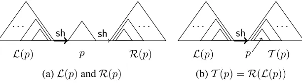
The set of all states with which a state p can legally reduce from the right is denotedL(p), orleft states. (see Figure 3 (a)) We call any stateq ∈ L(p) aleft stateofp. Thus each element of this set would have the following form:
L(hi, j, sd...s0i) ∆
={hh, i, s0d...s00i |
fk(s0k−1) =fk(sk), ∀k∈[1, d]} (1)
in which the span of the “left” state’s top tree ends where that of the “right” state’s top tree begins, and
fk(sk) =fk(sk0−1)for allk∈[1, d].
Similarly, the set of all states with which a statep can legally reduce from the left is denotedR(p), or
right states. (see Figure 3 (a)) For two statesp, q,
p∈ L(q)⇔q ∈ R(p)
3.2 Algorithm 1
We constrain the searching time with a polynomial bound by transforming the original search graph with exponentially many derivations into a graph with polynomial number of states.
In Algorithm 1, we maintain a chartCand a prior-ity queueQ, both of which are based on hash tables. Chart C can be formally defined as a function mapping from the space of states to the space of derivations:
C :S → D.
sh
statep:
h , j, sd...s0i: (c, )
hj, j+ 1, sd−1...s0, wji: (c+ξ,0)
j < n PRED
h , j, A→α.Bβi: (c, )
hj, j, B →.γi: (c+s, s) (B→γ)∈G
rex
stateq:
hk, i, s0d...s00i: (c0, v0)
statep:
hi, j, sd...s0i: ( , v) hk, j, s0d...s01, s00xs0i: (c0+v+δ, v0+v+δ)
q∈ L(p) COMP
hk, i, A→α.Bβi: (c0, v0) hi, j, Bi: ( , v)
[image:4.612.75.541.58.148.2]hk, j, A→αB.βi: (c0+v, v0+v)
Figure 2: Deductive systems for dynamic programming shift-reduce parsing (Huang and Sagae, 2010) (left, omitting reycase), compared to weighted Earley parsing (Stolcke, 1995) (right). Hereξ=scsh(p),δ=scsh(q) +screx(p),
s = sc(B → γ),Gis the set of CFG rules,hi, j, Biis a surrogate for anyhi, j, B→γ.i, and is a wildcard that matches anything.
. . .
L(p)
sh sh . . .
R(p)
p
. . .
L(p)
sh . . .
T(p)
p
(a)L(p)andR(p) (b)T(p) =R(L(p))
Figure 3: Illustrations of left statesL(p), right statesR(p), and left corner statesT(p). (a) Left statesL(p)is the set of states that can be reduced withpso thatp.s0will be the right child of the top tree of the result state. Right states R(p)is the set of states that can be reduced withpso thatp.s0will be the left child of the top tree of the result state. (b) Left corner statesT(p)is the set of states that have the same reducibility as shifted statep, i.e.,∀p0 ∈ L(p), we
have∀q∈ T(p), q∈ R(p0). In both (a) and (b), thicksharrow means shifts from multiple states; thinsharrow means shift from a single state.
We use C[p]to retrieve the derivation inC that is associated with statep. We sometimes abuse this notation to sayC[x]to retrieve the derivation asso-ciated with signatureef(x)for derivationx. This is fine since we know derivationx’s state immediately from the signature. We say statep ∈ C ifef(p) is associated with some derivation inC. A derivation x ∈ C if C[x] = x. ChartC supports operation PUSH, denoted asC[x]←x, which associate a sig-natureef(x)with derivationx.
Priority queueQis defined similarly asC, except that it supports the operation POPthat pops the high-est priority item.
Following Stolcke (1995) and Nederhof (2003), we use the prefix score and the inside score as the priority inQ:
x≺y ⇔x.pre < y.preor
(x.pre =y.preandx.ins < y.ins), (2)
Note that, for simplicity, we again ignore the spe-cial case when two derivations have the same prefix score and inside score. In practice for this case we
can pick either one of them. This will not affect the correctness of our optimality proof in Section 5.1.
[image:4.612.153.459.213.297.2]In the DP best-first parsing algorithm, once a derivationx is popped from the priority queue Q, as usual we try to expand it with shift and reduce. Note that both left and right reduces are between the derivation x of state p = [x]∼ and an in-chart derivationy of left stateq = [y]∼ ∈ L(p)(Line 10 of Algorithm 1), as shown in the deductive system (Figure 2). We call this kind of reductionleft expan-sion.
We further expand derivation x of state p with some in-chart derivationz of stater s.t. p ∈ L(r), i.e., r ∈ R(p) as in Figure 3 (a). (see Line 11 of Algorithm 1.) Derivationzis in the chart because it is the descendant of some other derivation that has been explored beforex. We call this kind of reduc-tionright expansion.
Algorithm 1Best-First DP Shift-Reduce Parsing.
LetLC(x)
∆
=C[L([x]∼)]be in-chart derivations of [x]∼’s left states
Let RC(x)
∆
= C[R(p)] be in-chart derivations of
[x]∼’s right states
1: functionPARSE(w0. . . wn−1)
2: C ← ∅ .empty chart
3: Q ← {INIT} .initial priority queue 4: whileQ 6=∅do
5: x←POP(Q)
6: ifGOAL(x)then returnx .found best parse 7: if[x]∼6∈C then
8: C[x]←x .addxto chart
9: SHIFT(x,Q)
10: REDUCE(LC(x),{x},Q) .left expansion
11: REDUCE({x},RC(x),Q) .right expansion
12: procedureSHIFT(x,Q)
13: TRYADD(sh(x),Q) .shift 14: procedureREDUCE(A, B,Q)
15: for(x, y)∈A×Bdo .try all possible pairs 16: TRYADD(rex(x, y),Q) .left reduce 17: TRYADD(rey(x, y),Q) .right reduce 18: functionTRYADD(x,Q)
19: if[x]∼6∈Qorx≺Q[x]then
20: Q[x]←x .insertxintoQor updateQ[x]
3.3 Algorithm 2: Lazy Expansion
We further improve DP best-first parsing with lazy expansion.
In Algorithm 2 we only show the parts that are different from Algorithm 1.
Assume ashiftedderivationxof statepis a direct descendant from derivationx0 of statep0, thenp ∈ R(p0), and we have:
∀ys.t.[y]∼=q∈REDUCE({p0},R(p0)), x≺y
which is proved in Section 5.1.
More formally, we can conclude that
∀ys.t.[y]∼ =q∈REDUCE(L(p),T(p)), x≺y
whereT(p)is theleft corner statesof shifted state p, defined as
T(hi, i+1, sd...s0i)=∆{hi, h, s0d...s
0
0i | fk(s0k) =fk(sk), ∀k∈[1, d]}
which represents the set of all states that have the same reducibility as a shifted statep. In other words,
T(p) =R(L(p)),
Algorithm 2Lazy Expansion of Algorithm 1.
LetTC(x)
∆
=C[T([x]∼)]be in-chart derivations of [x]∼’s left-corner states
1: functionPARSE(w0. . . wn−1)
2: C ← ∅ .empty chart
3: Q ← {INIT} .initial priority queue 4: whileQ 6=∅do
5: x←POP(Q)
6: ifGOAL(x)then returnx .found best parse 7: if[x]∼6∈C then
8: C[x]←x .addxto chart
9: SHIFT(x,Q)
10: REDUCE(x.lefts,{x},Q) .left expansion 11: else ifx.actionisshthen
12: REDUCE(x.lefts,TC(x),Q) .right expan.
13: procedureSHIFT(x,Q) 14: y←sh(x)
15: y.lefts ← {x} .initializelefts
16: TRYADD(y,Q) 17: functionTRYADD(x,Q) 18: if[x]∼∈Qthen
19: ifx.actionisshthen .maintainlefts
20: y←Q[x]
21: ifx≺ythenQ[x]←x 22: Q[x].lefts ←y.lefts∪x.lefts
23: else ifx≺Q[x]then
24: Q[x]←x
25: else . x6∈Q
26: Q[x]←x
which is illustrated in Figure 3 (a). Intuitively,T(p) is the set of states that havep’s top tree,p.s0, which
contains only one node, as the left corner.
Based on this observation, we can safely delay the REDUCE({x},RC(x))operation (Line 11 in Algo-rithm 1), until the derivation xof a shifted state is popped out fromQ. This helps us eliminate unnec-essary right expansion.
We can delay even more derivations by extending the concept of left corner states to reduced states. Note that for any two statesp, q, ifq’s top treeq.s0
hasp’s top treep.s0as left corner, andp,qshare the
same left states, then derivations ofpshould always have higher priority than derivations of q. We can further delay the generation ofq’s derivations until p’s derivations are popped out.2
2We did not implement this idea in experiments due to its
4 Comparison with Best-First CKY and Best-First Earley
4.1 Best-First CKY and Knuth Algorithm
Vanilla CKY parsing can be viewed as searching over a hypergraph(Klein and Manning, 2005), where a hyperedge points from two nodesx, yto one node z, ifx, ycan form a new partial tree represented by z. Best-first CKY performs best-first search over the hypergraph, which is a special application of the Knuth Algorithm (Knuth, 1977).
Non-DP best-first shift-reduce parsing can be viewed as searching over a graph. In this graph, a node represents a derivation. A node points to all its possible descendants generated from shift and left and right reduces. This graph is actually a tree with exponentially many nodes.
DP best-first parsing enables state merging on the previous graph. Now the nodes in the hyper-graph are not derivations, but equivalence classes of derivations, i.e., states. The number of nodes in the hypergraph is no longer always exponentially many, but depends on the equivalence function, which is the atomic feature functionef(·)in our algorithms.
DP best-first shift-reduce parsing is still a special case of the Knuth algorithm. However, it is more dif-ficult than best-first CKY parsing, because of the ex-tra topological order consex-traints from shift actions.
4.2 Best-First Earley
DP best-first shift-reduce parsing is analogous to weighted Earley (Earley, 1970; Stolcke, 1995), be-cause: 1) in Earley the PRED rule generates states similar to shifted states in shift-reduce parsing; and, 2) a newly completed state also needs to check all possible left expansions and right expansions, simi-lar to a state popped from the priority queue in Al-gorithm 1. (see Figure 2)
Our Algorithm 2 exploits lazy expansion, which reduces unnecessary expansions, and should be more efficient than pure Earley.
5 Optimality and Polynomial Complexity
5.1 Proof of Optimality
We define abest derivationof state[x]∼as a deriva-tionxsuch that∀y∈[x]∼,xy.
Note that each state has a unique feature signa-ture. We want to prove that Algorithm 1 actually fills the chart by assigning a best derivation to its state. Without loss of generality, we assume Algorithm 1 fillsC with derivations in the following order:
x0, x1, x2, . . . , xm
wherex0is the initial derivation,xmis the first goal
derivation in the sequence, andC[xi] =xi,0≤i≤
m. Denote the status of chart right after xk being
filled asCk. Specially, we defineC−1=∅
However, we do not have superiority as in non-DP best-first parsing. Because we use a pair of prefix score and inside score,(pre,ins), as priority (Equa-tion 2) in the deductive system (Figure 2). We have the following property as an alternative for superior-ity:
Lemma 1. After derivation xk has been filled into chart, ∀x s.t. x ∈ Q, and x is a best derivation of state [x]∼, then x’s descendants can not have a
higher priority thanxk.
Proof. Note that whenxk pops out, xis still in Q,
soxkx. Assumezisx’s direct descendant.
• Ifz = sh(x) orz = re(x, ), based on the de-ductive system,x≺z, soxk x≺z.
• Ifz=re(y, x),y∈ L(x), assumez≺xk.
z.pre =y.pre+y.sh+x.ins+x.re
We can construct a new derivationx0 ∼ x by appendingx’s top tree,x.s0 toy’s stack, and
x0.pre =y.pre+y.sh+x.ins< z.pre
Sox0 ≺z ≺xk x, which contradicts thatx
is a best derivation of its state.
With induction we can easily show that any descen-dants ofxcan not have a higher priority thanxk.
We can now derive:
Theorem 1 (Stepwise Completeness and Optimal-ity). For anyk,0≤ k≤m, we have the following two properties:
Proof. We prove by induction onk.
1. Fork= 0, these two properties trivially hold.
2. Assume this theorem holds fork= 2, ..., i−1. Fork=i, we have:
a) [Proof for Stepwise Completeness]
(Proof by Contradiction) Assume ∃x ≺ xi
s.t.[x]∼ 6∈ Ci−1.Without loss of generality we
take a best derivation of state[x]∼asx.xmust be derived from other best derivations only. Consider this derivation transition hypergraph, which starts at initial derivationx0 ∈Ci−1, and
ends atx6∈Ci−1.
There must be a best derivationx0 in this tran-sition hypergraph, s.t. all best parent deriva-tion(s) ofx0are inCi−1, but notx0.
Ifx0 is a reduced derivation, assume x0’s best parent derivations are y ∈ Ci−1, z ∈ Ci−1.
Becauseyandzare best derivations, and they are inCi−1, from Stepwise Optimality onk= 1, ..., i−1, y, z ∈ {x0, x1, . . . , xi−1}. From
Line 7-11 in Algorithm 1, x0 must have been pushed intoQwhen the latter ofy, zis popped.
Ifx0 is a shifted derivation, similarly x0 must have been pushed intoQ.
Asx0 6∈Ci−1,x0 must still be inQ whenxiis
popped. However, from Lemma 1, none ofx0’s descendants can have a higher priority thanxi,
which contradictsx≺xi.
b) [Proof for Stepwise Optimality]
(Proof by Contradiction) Assume ∃x ∼ xi
s.t.x ≺ xi. From Stepwise Completeness on
k = 1, ..., i,x ∈ Ci−1, which means the state [xi]∼ has already been assigned to x, contra-dicting the premise thatxiis pushed into chart.
Both of the two properties have very intuitive meanings. Stepwise Optimality means Algorithm 1 only fills chart with a best derivation for each state. Stepwise Completeness means every state that has its best derivation better than best derivationpimust
have been filled before pi, this guarantees that the
rex
hh00, h0
k...i
i: (c0, v0) hh0, h
i...j
i: ( , v)
hh00, h
k...j
[image:7.612.318.514.61.152.2]i: (c0+v+λ, v0+v+λ)
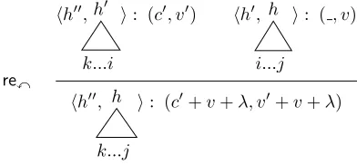
Figure 4: Example of shift-reduce with dynamic pro-gramming: simulating an edge-factored model. GSS is implicit here, and rey case omitted. Here λ =
scsh(h00, h0) +screx(h
0, h).
global best goal derivation is captured by Algo-rithm 1.
More formally we have:
Theorem 2 (Optimality of Algorithm 1). The first goal derivation popped off the priority queue is the optimal parse.
Proof. (Proof by Contradiction.) Assume∃x, x is the a goal derivation andx ≺ xm. Based on
Step-wise Completeness of Theorem 1,x∈Cm−1, thusx
has already been popped out, which contradicts that xmis the first popped out goal derivation.
Furthermore, we can see our lazy expansion ver-sion, i.e., Algorithm 2, is also optimal. The key ob-servation is that we delay the reduction of derivation x0 and a derivation of right statesR([x0]∼)(Line 11 of Algorithm 1), until shifted derivation,x=sh(x0), is popped out (Line 11 of Algorithm 2). However, this delayed reduction will not generate any deriva-tion y, s.t. y ≺ x, because, based on our deduc-tive system (Figure 2), for any such kind of reduced derivationsy,y.pre=x0.pre+x0.sh+y.re+y.ins, whilex.pre =x0.pre+x0.sh.
5.2 Analysis of Time and Space Complexity
Following Huang and Sagae (2010) we present the complexity analysis for our DP best-first parsing.
Theorem 3. Dynamic programming best-first pars-ing runs in worst-case polynomial time and space, as long as the atomic features function satisfies:
• bounded: ∀derivationx,|ef(x)|is bounded by
a constant.
– horizontal: ∀k, fk(s) = fk(t) ⇒ fk+1(s) = fk+1(t), for all possible trees
s,t.
– vertical: ∀k, fk(sys0) = fk(tyt0) ⇒ fk(s) =fk(t)andfk(sxs0) =fk(txt0)⇒ fk(s0) =fk(t0), for all possible treess,s0,
t,t0.
In the above theorem, boundness means we can only extract finite information from a derivation, so that the atomic feature function ef(·) can only dis-tinguish a finite number of different states. Mono-tonicity requires the feature representation fk sub-sumes fk+1. This is necessary because we use the
features as signature to match all possible left states and right states (Equation 1). Note that we add the vertical monotonicity condition following the sug-gestion from Kuhlmann et al. (2011), which fixes a flaw in the original theorem of Huang and Sagae (2010).
We use the edge-factored model (Eisner, 1996; McDonald et al., 2005) with dynamic programming described in Figure 4 as a concrete example for com-plexity analysis. In the edge-factored model the fea-ture set consists of only combinations of informa-tion from the roots of the two top trees s1, s0, and
the queue. So the atomic feature function is
ef(p) = (i, j, h(p.s1), h(p.s0))
whereh(s)returns the head word index of trees. The deductive system for the edge-factored model is in Figure 4. The time complexity for this deduc-tive system is O(n6), because we have three head indexes and three span indexes as free variables in the exploration. Compared to the work of Huang and Sagae (2010), we reduce the time complexity from O(n7) to O(n6) because we do not need to keep track of the number of the steps for a state.
6 Experiments
In experiments we compare our DP best-first parsing with non-DP best-first parsing, pure greedy parsing, and beam parser of Huang and Sagae (2010).
Our underlying MaxEnt model is trained on the Penn Treebank (PTB) following the standard split: Sections 02-21 as the training set and Section 22 as the held-out set. We collect gold actions at differ-ent parsing configurations as positive examples from
model score accuracy # states time greedy −1.4303 90.08% 125.8 0.0055
beam∗ −1.3302 90.60% 869.6 0.0331
non-DP −1.3269 90.70% 4,194.4 0.2622
[image:8.612.317.542.58.118.2]DP −1.3269 90.70% 243.2 0.0132
Table 1: Dynamic programming best-first parsing reach optimality faster. *: for beam search we use beam size of 8. (All above results are averaged over the held-out set.)
gold parses in PTB to train the MaxEnt model. We use the feature set of Huang and Sagae (2010).
Furthermore, we reimplemented the beam parser with DP of Huang and Sagae (2010) for compari-son. The result of our implementation is consistent with theirs. We reach 92.39% accuracy with struc-tured perceptron. However, in experiments we still use MaxEnt to make the comparison fair.
To compare the performance we measure two sets of criteria: 1) the internal criteria consist of the model score of the parsing result, and the number of states explored; 2) the external criteria consist of the unlabeled accuracy of the parsing result, and the parsing time.
We perform our experiments on a computer with two 3.1GHz 8-core CPUs (16 processors in total) and 64GB RAM. Our implementation is in Python.
6.1 Search Quality & Speed
We first compare DP best-first parsing algorithm with pure greedy parsing and non-DP best-first pars-ing without any extra constraints.
The results are shown in Table 1. Best-first pars-ing reaches an accuracy of 90.70% in the held-out set. Since that the MaxEnt model is locally trained, this accuracy is not as high as the best shift-reduce parsers available now. However, this is sufficient for our comparison, because we aim at improving the search quality and efficiency of parsing.
Compared to greedy parsing, DP best-first pars-ing reaches a significantly higher accuracy, with∼2 times more parsing time. Given the extra time in maintaining priority queue, this is consistent with the internal criteria: DP best-first parsing reaches a significantly higher model score, which is actually optimal, exploring twice as many as states.
0 0.02 0.04 0.06 0.08 0.1 0.12
0 10 20 30 40 50 60 70
avg. parsing time (secs)
sentence length non-DP
[image:9.612.73.299.62.221.2]DP beam
Figure 5: DP best-first significantly reduces parsing time. Beam parser (beam size 8) guarantees linear parsing time. Non-DP best-first parser is fast for short sentences, but the time grows exponentially with sentence length. DP best-first parser is as fast as non-DP for short sentences, but the time grows significantly slower.
However, it explores∼17 times more states than DP, with an unbearable average time.
Furthermore, on average our DP best-first parsing is significantly faster than the beam parser, because most sentences are short.
Figure 5 explains the inefficiency of non-DP best-first parsing. As the time complexity grows expo-nentially with the sentence length, non-DP best-first parsing takes an extremely long time for long sen-tences. DP best-first search has a polynomial time bound, which grows significantly slower.
In general DP best-first parsing manages to reach optimality in tractable time with exact search. To further investigate the potential of this DP best-first parsing, we perform inexact search experiments with bounded priority queue.
6.2 Parsing with Bounded Priority Queue
Bounded priority queue is a very practical choice when we want to parse with only limited memory.
We bound the priority queue size at 1, 2, 5, 10, 20, 50, 100, 500, and 1000, and once the priority queue size exceeds the bound, we discard the worst one in the priority queue. The performances of non-DP best-first parsing and non-DP best-first parsing are illustrated in Figure 6 (a) (b).
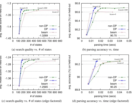
Firstly, in Figure 6 (a), our DP best-first pars-ing reaches the optimal model score with bound
50, while non-DP best-first parsing fails even with bound 1000. Also, in average with bound 1000, compared to non-DP, DP best-first only needs to ex-plore less than half of the number of states.
Secondly, for external criteria in Figure 6 (b), both algorithms reach accuracy of 90.70% in the end. In speed, with bound 1000, DP best-first takes ∼1/3 time of non-DP to parse a sentence in average.
Lastly, we also compare to beam parser with beam size 1, 2, 4, 8. Figure 6 (a) shows that beam parser fails to reach the optimality, while exploring signif-icantly more states. On the other hand, beam parser also fails to reach an accuracy as high as best-first parsers. (see Figure 6 (b))
6.3 Simulating the Edge-Factored Model
We further explore the potential of DP best-first parsing with the edge-factored model.
The simplified feature set of the edge-factored model reduces the number of possible states, which means more state-merging in the search graph. We expect more significant improvement from our DP best-first parsing in speed and number of explored states.
Experiment results confirms this. In Figure 6 (c) (d), curves of DP best-first diverge from non-DP faster than standard model (Figure 6 (a) (b)).
7 Conclusions and Future Work
We have presented a dynamic programming algo-rithm for best-first shift-reduce parsing which is guaranteed to return the optimal solution in poly-nomial time. This algorithm is related to best-first Earley parsing, and is more sophisticated than best-first CKY. Experiments have shown convincingly that our algorithm leads to significant speedup over the non-dynamic programming baseline, and makes exact search tractable for the first-time under this model.
-1.45 -1.4 -1.35 -1.3
0 100 200 300 400 500 600 700 800 900
avg. model score on held-out
# of states
bound=50 bound=1000
beam=8
non-DP DP beam -1.3269
90 90.2 90.4 90.6 90.8
0 0.01 0.02 0.03 0.04 0.05
avg. accuracy (%) on held-out
parsing time (secs)
bound=50
bound=1000
beam=8
non-DP DP beam 90.70
(a) search quality vs. # of states (b) parsing accuracy vs. time
-1.4 -1.36 -1.32 -1.28 -1.24
0 100 200 300 400 500 600 700 800 900
avg. model score on held-out
# of states
bound=20 bound=500 beam=8
non-DP DP beam -1.2565
89.8 90 90.2
0 0.01 0.02 0.03 0.04 0.05
avg. accuracy (%) on held-out
parsing time (secs)
bound=20 bound=500
beam=8
non-DP DP beam 90.25
[image:10.612.82.541.168.525.2](c) search quality vs. # of states (edge-factored) (d) parsing accuracy vs. time (edge-factored)
References
Alfred V. Aho and Jeffrey D. Ullman. 1972. The The-ory of Parsing, Translation, and Compiling, volume I: Parsing ofSeries in Automatic Computation. Prentice Hall, Englewood Cliffs, New Jersey.
Sharon A Caraballo and Eugene Charniak. 1998. New figures of merit for best-first probabilistic chart pars-ing. Computational Linguistics, 24(2):275–298. Jay Earley. 1970. An efficient context-free parsing
algo-rithm. Communications of the ACM, 13(2):94–102. Jason Eisner. 1996. Three new probabilistic models for
dependency parsing: An exploration. InProceedings of COLING.
Liang Huang and Kenji Sagae. 2010. Dynamic program-ming for linear-time incremental parsing. In Proceed-ings of ACL 2010.
Dan Klein and Christopher D Manning. 2003. A* pars-ing: Fast exact Viterbi parse selection. InProceedings of HLT-NAACL.
Dan Klein and Christopher D Manning. 2005. Pars-ing and hypergraphs. InNew developments in parsing technology, pages 351–372. Springer.
Donald Knuth. 1977. A generalization of Dijkstra’s al-gorithm. Information Processing Letters, 6(1). Marco Kuhlmann, Carlos G´omez-Rodr´ıguez, and
Gior-gio Satta. 2011. Dynamic programming algorithms for transition-based dependency parsers. In Proceed-ings of ACL.
Ryan McDonald, Koby Crammer, and Fernando Pereira. 2005. Online large-margin training of dependency parsers. InProceedings of the 43rd ACL.
Mark-Jan Nederhof. 2003. Weighted deductive pars-ing and Knuth’s algorithm. Computational Linguis-tics, pages 135–143.
Joakim Nivre. 2008. Algorithms for deterministic incre-mental dependency parsing. Computational Linguis-tics, 34(4):513–553.
Adam Pauls and Dan Klein. 2009. Hierarchical search for parsing. In Proceedings of Human Language Technologies: The 2009 Annual Conference of the North American Chapter of the Association for Com-putational Linguistics, pages 557–565. Association for Computational Linguistics.
Kenji Sagae and Alon Lavie. 2006. A best-first proba-bilistic shift-reduce parser. InProceedings of ACL. Andreas Stolcke. 1995. An efficient probabilistic
context-free parsing algorithm that computes prefix probabilities. Computational Linguistics, 21(2):165– 201.