Infinite sets of polynomial conserved densities for nonlinear evolution equations

POLYNOMIAL CONSERVED DENSITIES FOR

NONLINEAR EVOLUTION EQUATIONS

A thesis

submitted in p~rtial fulfilment of the requirements for the Degree

of

Doctor of Philosophy in Physics in the

University of Canterbury

by

Mark J. McGuinness

CHAPTER

·ABSTRACT

I. INTRODUCTION

NOETHER'S THEOREM •

1. The Variation of the Action Integral

2. Hamilton's Principle and the Euler-Lagrange Equation of Motion

3. Noether's Theorem

4. Conventional Noether's Theorem

5. An Alternative Approach to Noether's Theorem 6. Generalised Noether's Theorem

7. The Noether Family of Transformations

II. THE KORTEWEG-DE VRIES EQUATION

1. Dackg:rcund

2. The Inverse Spectral Method of Solution •

3. Soliton Solutions . • • • 4. Backlund Transformations

5. The Generalised KdV Equations

6. An Infinite Set of Conservation Laws

7. Conserved Densities of the KdV Equation Identified as Energy Dens i ti.es

8. Corollary for Generalised KdV Equations

9. Conserved Densities of the KdV Equation Identified as Momentum Densities

10. Application to the Linearised KdV Equation

IV. THE MODIFIED KORTEWEG-DE VRIES EQUATION • 1. Bqckground

2. Backlund Transformations and Conservation Laws 3. Conserved Densities of the Modified KdV Equation

Identified as Energy Densities • .

4. Conserved Densities of the Modified KdV Equation Identified as Momentum Densities

1. The Conserved Densities of the Sine-Gordon Equation Identified as Momentum Densities

2. The Energy Densities of the Higher-Order Sine-Gordon Equations

3 • . A Correspondence Between the Conserved Densities of the

124

138

Sine-Gordon and the Modified KdV Equation • • • . • 142

VI. THE CLASSICAL NONLINEAR SHALLOW-WATER EQUATIONS •

1.· An Infinite set of Conserved Energy Densities for the Classical Shallow-Water Equations • •

2. An Infinite Set of Conserved Momentum Densities for the Classical Shallow-Water Equations

VII CONCLUSIONS

1. The Linear Case • 2. Generalisation

ACKNOWLEDGEMENTS

REFERENCES

APPENDICES

145

146

159

161 162 164

172

173

FIGURE 2.1 2.2

A Schematic of the Development of Chapter II

The Variations o¢,8¢, for a Transformation (ox,o¢) • • 2.3 A Schematic of the Relationships Between Requirement (B),

Invariance Transformations₁and Symmetry Transformations • 2.4 Schematic of Relationships Between Different Approaches to

PAGE 12 17

32

Noether'sTheorem and the Noether Family of Transformations 48

2.5 The Active and Passive Views of an x-Translation

3.1 Diagram of the Inverse Spectral Method for Solving the KdV Equation

3.2 The Extended Backlund Transformations .

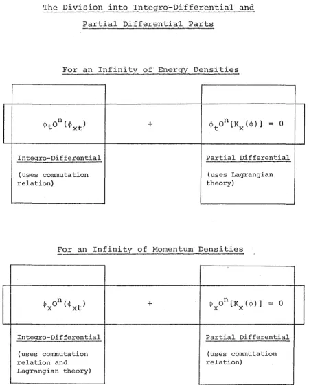
7.1 The Division into Integra-Differential and Partial Differ-ential Parts

50

60 70

The infinite sets of polynomial conserved densities which have been found for the Korteweg-de Vries equation, the modified Korteweg-de Vries equation, the Sine-Gordon

equation, and the classical nonlinear shallow-water equations, are investigated using Noether's theorem. These sets are

identified

as energy or momentum densities of sets of

CHAPTER I INTRODUCTION

Conservation laws have always been useful in helping to understand and solve the equations governing some system, and have played a part in the progress made in recent years in the attempt to solve certain nonlineaP evolution equations. These nonlinear equations have possessed some remarkable

features, including the existence of soliton solutions, which are solitary wave solutions whose shape and velocity are preserved after a collision with each other, the

existence of a linear scattering technique for solving exactly the initial boundary-value problem, the existence of B§cklund transformations mapping solutions to solutions, and the existence of an infinite numbeP of eonsePvation laws.

Since Noether's (1918) theorem, i t has proved interesting and fruitful to relate the aonsePvation laws of a system

with the symmetPies of that system. The symmetries of a

system, in classical Lagrangian theory, are continuous groups of transformations leaving the action integral invariant. Noether's theorem associates these transformations with

conservation laws of the system. By using Noether's theorem, i t is possible to identify conservation laws by their associated transformation, and to pPediet conservation laws from the

existence of the symmetry.

The existence of an infinite number of conservation

situation, this thesis will investigate such sets of conser-vation laws for several nonlinear evolution equations, using Noether's theorem. The conservation laws investigated will be

identified

as being equivalent to energy or momentum conservation laws for higher-order nonlinear equations, whose solution sets contain that of the nonlinear evolution equation under consideration. In. the concluding chapter, a general technique with possibilities for

predicting

such infinite sets of conservation laws for other nonlinear equations will be presented.

Infinite sets of polynomial conserved densities [poly-nomials in the field variables and their derivatives] are easily derived for

linear

evolution equations. For example, the classical linear wave equation

is derivable from the Lagrangian

L = - ~~ ~ _{t t} + ~~ ~ _{X X}

Differentiating equation (1.0.1) n times with respect to x gives

Substituting

(1.0.1)

(1.0.2)

(1.0.3)

in equation (1.0.3) yields

(1.0.5)

with the Lagrangian

L

=

(1.0.6)

Since the Lagrangians (1.0.6) have no explicit dependence on time or space variables, Noether's theorem implies that

energy and momentum are conserved for equations (1.0.5) for any n. Since solutions to equation (1.0.1) must also be solutions to equations (1.0.5), these energies and momenta constitute an infinite set of polynomial conserved densities for equation (1.0.1).

From an alternative point of view, using Rosen's general-ised Noether's theorem, an equivalent set of energies and momenta may be obtained by differentiating equation (1.0.1)

2n times with respect to x, and multipling by ¢t (for energy), or

¢

[for momentum].

X

This approach can be generalised to vector f ld variables and several dimensions. One notable example is the derivation by Steudel (1965), who gives a generalised version of the

preceding argument, and shows that such an argument explains Kibble's (1965) infinite number of conservation of

ziZah

equations for electromagnetic fields.

of the motion, i t is not surprising that such an equation should possess an infinite number of conservation laws. This view applies whether the discrete system is linear or nonlinear, and hence there is no reason to believe that nonlinearity will prevent continuous wave equations from possessing infinite numbers of conservation laws. What is

not

clear is whether such laws will yield conserved densities in tractable form.

The above approach, of operating n times with a differential operator, fails when applied to

nonZinear

equations, as equations of the same form [such as equation (1.0.5)] do not follow

from a nonlinear equation. The thrust of this investigation has been to show that more sophisticated operators, acting repeatedly on the nonlinear evolution equations under con-sideration, yield higher-order equations with polynomial conserved energy or momentum densities. Such operators have been found for several nonlinear wave equations of current

interest, giving some insight into the form of these operators, which have been nonlinear and integra-differential in nature.

It has not been possible to obtain general principles for the formation of such operators for arbitrary nonlinear wave

equations, although general properties of these operators are pointed out.

Noether's theorem is reviewed in depth in chapter 2,

because of the major part i t has played in the discovery of these properties.

Summaries of some of Steudel's work are to be found in sections (3.6) and (4.2). Steudel has successfully used

Noether's theorem to relate the infinite sets of conservation laws of the KdV and the modified KdV equations to infinitesimal extended Backlund transformations. The remainder of this

thesis is original material.

Sections (3.7) and (3.9) identify the infinite set of polynomial conserved densities obtained by Gardner, Greene, Kruskal and Miura (1974) for the KdV equation as energy or

momentum densities of higher-order integra-differential envelop-ing KdV equations, usenvelop-ing Noether's theorem. Section (3.8)

presents a corollary for the generalised KdV equations. An application to the linearised KdV equation is given in

section (3.10).

In chapter 4, Noether's theorem is used to identify the infinite set of polynomial conserved densities for the

modified KdV equation as equivalent to energy or momentum densities of higher-order modified KdV equations, whose solution sets contain that of the modified KdV equation.

The Sine-Gordon equation, which also possesses an

The technique of previous chapters is extended to a

matrix

formalism in chapter 6, and is used to identify an infinite set of polynomial conserved densities for the classical nonlinear shallow-water equations as energy or momentum densities of higher-order equations.

CHAPTER II NOETHER'S THEOREM

Noether's theorem [Noether, (1918)] provides a natural way of associating a conserved quantity for a system with an infinitesimal transformation on that system. This association can serve as a means of identifying the conserved quantity. For example, conservation of energy or momentum is associated with invariance of the system under an infinitesimal time or space translation, conservation of angular momentum is

associated with invariance under an infinitesimal rotation, and conservation of charge is associated with invariance under an infinitesimal phase or gauge transformation of the field variables. Noether's theorem also provides a general framework for predicting which systems or equations will have a certain type of conservation law. For example, if the Lagrangian density for a system has no explicit

time-dependence, Noether's theorem says that energy is conserved in that system [see appendix C] •

A brief statement of the theorem is presented here. Define the action integral

J _

J

L dx

v

over a volume v in four-space, where L is the Lagrangian

(2.0.1)

in terms of which the equation of motion for a system

may be expressed, as will be seen in section (2.2).

Noether's t theorem says that

i f the action

:1.

integraZ

J

is invariant under the infinitesimat

one-parameter transformation

say

X1

=

X + OX(X)

¢' (x) = ¢ (x)

+

'8¢ (x)

'

oJ

=

J

(-d

G~)dx

,

v ).l

where

GJ.l

is zero on the boundary of voZume

v

so that

oJ

is

zero~

then the foZtowing reZation

[Noether's

relation]

hoZds:

where

I

a=l

a

1:

I

a=O b=O

and

d

lla

[_oL_l,

_o¢~1

•••

~a

d •••

lll d _~b [ _ _ a_L - - ] d •••

The operator E is known as the Euler-Lagrange operator. Note that repeated indices are summed upon and can be

treated as dummy indices, and that dv is a total derivative whereas avis a partial ~erivative, regarding ~(x) as

independent of xv. That is, av is a derivative with respect to expZicit xv - dependence [not via ~].

Noether's relation (2.0.4) associates the variation

(8~,ox) with the conservation equation

This is because, as will be seen in section (2.2),

is the equation of motion for the system with action integral

J.

(2.0.7)

(2.0.8)

The variation (6~,ox) is an invariance transformation in the sense that J is functionally invariant under it.

her's theorem in physics. Rosen (1971) gives a icularly good account of conventional formulations be theorem; Hill (1951) has a clear derivation; ~der (1968) gives a clear statement of the original theorem; Trautman (1967) has a mathematically rigorous treatment; Boyer (1966, 1967), Dass {1966) and Dothan

(1972) also have interesting approaches to the theorem. These differing approacr l interpretations can be confusing to the uninitiated. This chapter attempts to present a unified account of these approaches,

discussing their advantages and disadvantages.

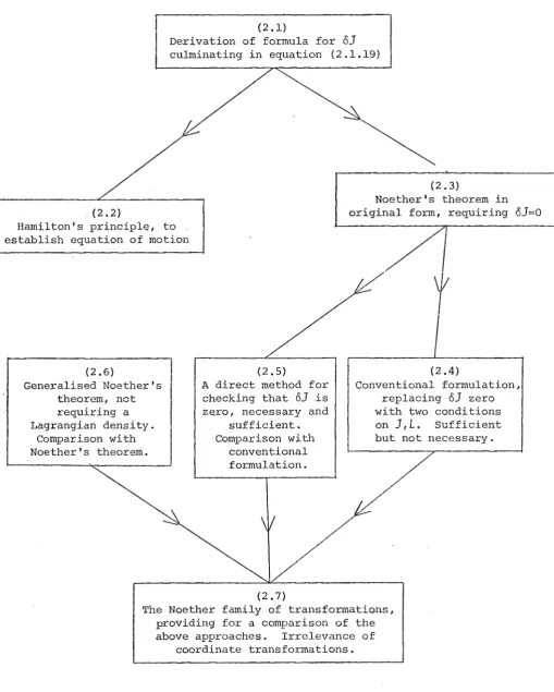
The organisation of this chapter is presented in flow chart form in figure (2.1), to help clarify the

development. In section (2.1), a mathematical formula will be derived for the functional variation of the action integral

J

under the infinitesimal transformation (6¢,ox). This formula is fundamental to the proof of Noether's theorem.

A brief excursion is made into Hamilton's principle in section (2.2), to establish.the equations of motion for a system.

FIGURE (2.1)

A Schematic of the Development of Chapter II

(2 .1)

Derivation of formula for

oJ

culminating in equation (2.1.19)

( 2. 3)

. (2.2)

Hamilton's principlq, to . establish equation of motion

Noether's theorem in original form, requiring

81=0

(2. 6)

Generalised Noether's theorem, not requiring a Lagrangian density.

Comparison with Noether's theorem.

{ 2. 5}

A direct method for checking that

6J

is zero, necessary and

sufficient. Comparison with

conventional formulation.

(2. 7)

{2.4)

Conventional formulation, replacing

oJ

zero with two conditions

on

J,L.

Sufficient

but not necessary.

The Noether family of transformations, providing for a comparison of the above approaches. Irrelevance of

[image:17.595.45.555.148.784.2]

physical implication. However, these requirements are sufficient but not necessary for

oJ

to be zero. An alternative approach, sufficient and. necessary for

oJ

to be zero, is presented in section (2.5}. It is shown that this approach yields a more direct method for

checking that 81 is zero, than that in section (2.4}.

In section (2.6) a quite different approach to conservation laws is presented. Called generalised Noether's theorem, this approach does not explicitly require a Lagrangian density, but does require the equation of motion. This can be of some advantage as some equations do not have Lagrangian densities. Tpis approach uses a relation

similar to Noether's relation (2.0.4) as a starting point, rather than using the expression derived for oJ in section

(2.1). Generalised Noether's theorem is shown to be mathematically equivalent to Noether's theorem if a

Lagrangian density exists for the system. In section (2.7), the concept of a Noether family of transformations (o~,ox) is introduced, facil·itating a comparison of the three

approaches to Noether's theorem.

(2.1) THE VARIATION OF THE ACTION INTEGRAL

The derivation of Noether's theorem involves the determination of the functional variation of the action integral

where the Lagrangian density

is a function of the independent variables [coordinates]

x~ and of the dependent or field variable ~ and its derivatives to any order. This function characterises any system described by an Euler-Lagrange equation of motion, as is shown in section (2.2). A system may

have several Lagrangians and several eld variables, and

(2.1.2)

the field variables may be tensor quantities. For clarity and ease of notation this derivation will deal with one Lagrangian density depending on one scalar field variable and any number of derivatives of that variable. The

generalisation to several Lagrangians, several field variables and tensor quantities is easily made.

The functional variation of the action integral under the infinitesimal transformation

OX - X1

- X= OX(X) (2.1.3)

o~

-

~' (x') - ~ (x)

is defined as

o.7 -

f

L(x'

,~·

(x') I • • • )dx' -

J

L(x,cfl(x) I • • • )dx

v'

· v

where v 1 _{is the transformation of the four-volume v under}

ox. ox will be treated as a function of x only, although i t can be generalised to a function of x and ¢ and its derivatives [e.g., Dothan (1972)].

J will be expressed in the form of a four-divergence term and a remainder term, using the infinitesimal nature of the transformation, and retaining only terms that are up to first-order in the transformation.

To first-order in the variation,

dx1

=

dx1

dy1

dz1

dt1

=

[1

+

d~(ox~)]dx .(2.1.5)

so that

oJ

=

J

{L[x1

] - L[x] + L[x1 ] d

(ox~)}dx

v ~

·where

L [xI] - L (xI' ¢I (xI)' ..• )

Using a Taylor expansion,

L[x1

] - L[x]

= ()

L

ox~

+

I

CJx~ _a CJL

o¢~1

•••

~a

CJ¢~1

• •.

~a

where the sum is over combinations of { ~ 1 , • • • , ~ } •

a To first order in the variation,

(2.1.6)

(2.1.7)

so that using equations (2.1.7) and (2.1.8), equation (2.1.6} becomes

oJ

=

fv

n:

a ()<j>lll

aL

.

.

.

(2.1.9)

It is useful here to define ·a different field variation to that used so far,

5¢ (x) - <j>' (x) - ¢ (x)

The definitions of the field variations can be used to show that

'

to first order in the variations. Hence, either {o¢,ox) or (8¢,ox) is sufficient to define the variation or

transformation used.

(2.1.10)

(2.1.11)

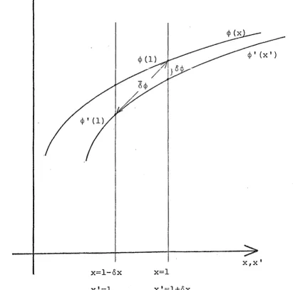
The first field variation¢' (x') - ¢(x) can be viewed as the change in the field variable

at a fixed point in

spaae~ that point having the coordinates {x) in the

untransformed system and (x') in the transformed system. In this sense, o¢ is the true change in the field ¢ at a point.

The second field variation ¢' (x) - ¢(x) is the change in ¢

at a fixed grid referenae point or set of

FIGURE (2.2}

iations

o

Transformation

x=l-ox

x'=l

for a

x=l

x'=l+ox

[image:22.597.125.537.301.708.2]

fixed in space under the transformation, since the

trans-formation may explicitly change the coordinate system.

See figure (2.2) for a pictorial representation of o¢,

6¢ for the case of a variation ox in a single x - coordinate

and a field variation o¢ which is nonzero.

The advantage of using 6¢ instead of o¢ is that 6

commutes with differentiation, that is

(2.1.12)

whereas, realising that the definitions for o¢ and 6¢

also apply When

¢

is replaced by ¢ ,

J.ll . . . J.l a

dJ.l(o¢)

=

d [¢'(x') - ¢ (x)] _].l

v'

d _[¢'(x')] dx

- <P (x)

=

--v-,

dxJ.l ].l dx

=

<P'(x')[oJ.l

_v

_v

+ d (oxv)] - <flu(x)

].l

=

0 (¢].1) + <P

_v

dJ.l(oxv)

to first order in oxJ.l.

Realising that <P can be replaced by <P J.ll equation (2.1.11), equation (2.1.9) becomes

• • • ].l

a

+ ~

aL

~

].l /... 't'J.ll

...

a a 3¢

J.ll • • • J.la

(2.1.13)

in

oxv +

••• ].l v

+

~

oxl-l

+

Ld,₁(oxJJ)]dx,

dXjJ '"'

=

Jv

ri __

a_L __

6¢111 a a¢111 ••• 11a

(2.1.14)

••• (2 .1.15)

Using the commutative property (2.1.12), i t can be shown that

I _

___;.a_L _ _ 8¢111 a aq>l-ll _{••• JJa}

...

where it will be recall.ed that

E¢ ( L) 3:

I

(-1) a d • • • d

a=O 111 .

1T11 (t)8cp

-

I I

(-l)b d

a=O b=O 111

[ dL

11a _Clcpl-ll

. .

.

[ dL

d 11b

Clcp11l-ll

...

~

a

l

'

~

J

a d

11b+l

(2.1.16)

(2.1.17)

d

o¢ ,

11a

(2.1.18)

[see appendix A]. Substituting this result into equation

(2.1.15) gives the desired form for the functional variation of the action integral:

{2.1.19)

Equation (2.1.19) is the key equation for the derivation of the Euler-Lagrange equation of motion from Hamilton's

(2.2) HAMILTON'S PRINCIPLE AND THE EULER-LAGRANGE EQUATION OF MOTION

The generalisation of Hamiltons principle to field theory can be expressed as [Saletan and Cromer, (1971)]:

The true physical field variables are those with the

[arbitrary] required boundary values for whioh the aation

integral

J

is an extremum.

In other words, for a field variation

~·

=

~

+

0~ = ~

+

0~

with the restriction that a~ be zero on the boundary of integration in

J,

Hamilton's principle says that for

solutions,

oJ

must be zero. The restriction on 6¢ ensures that the boundary values of

¢

are fixed.

If

oJ

is zero, equation (2.1.19) becomes

(2.2.1)

using the divergence theorem, where B is the boundary of

v and dcr~ is an element on that surface. Hamilton's principle requires that

ox

be zero everywhere and 6¢ be zero on B, so that equation (2.2.1) becomes

(2.2.2)

E<j>(L)

=

0 (2.2.3)

for solutions of the system. This is the Euler-Lagrange equation of motion for the system.

For the Lagrangian density

(2.2.4)

for example, the Euler-Lagrange equation of motion is

d [aL

l

+ 'dL

=

0

- dxll

a¢

8;

ll

(2.2.5)

This derivation is reversible, so that Hamilton's principle is obeyed if and only if the Euler-Lagrange

equation holds. The generalization to systems with several equations of motion and with tensor field variables is

easily made.

In practice, the equation of motion for a system is often known, and is cast into the Euler-Lagrange form to obtain.a Lagrangian density for that system.

(2.3) NOETHERB THEOREM

Noether's first theorem will now be proved. If

oJ

is

zero~

equation (2.1.19) becomes

This is true if and only if the integrand is

(2.3.2)

where G~ is zero on the boundary B of V, since the divergence theorem then gives

(2.3.3)

It should be noted that the boundary of v is usually chosen such that

¢

and its derivatives are zero everywhere on it.

~ .

Then any function G (¢,¢~,

... )

will be zero on that boundary.

Clearly, equation (2.3.2) can be rearranged to give

Noether's relation:

(2.3.4)

and Noether's theorem is proved, as stated at the beginning of this chapter.

The connection between Noether's relation and the existence of a conserved quantity will now be established. Recall the equation of motion for a system from section (2.2),

(2.3.5)

for solutions to the equation of motion. An equation of this form, equating a four-divergence to zero, is known as a conservation equation or a conservation Zaw. This is because, under an assumption which is quite acceptable physically, such an equation gives rise to a conserved quantity, that is, something which does not change with time.

To see this, a distinction is made between time and space coordinates, so that equation (2.3.6) is written as

dt[7rt(L)8¢ +Lot+ Gt]

+~

.. a [7ra(L)8¢ + Loxa + Ga]

=

0, (2.3.7}

'-""'

where

xa

=

x,y,z and a

=

1,2,3

Integrating this equation over a three-space volume R and using the divergence theorem, i t becomes

dt JR [7rt(L}8¢ + Lot+

Gt]~

+

Ts

[7ra(L)8¢ + Loxa + Ga] daa

=

o .

(2.3.8) The assumption is made here that R can be chosen such that

then is that for any physical system, the field variable and its derivatives vanish if one goes far enough away from the system.

Under this assumption, the surface integral in equation (2.3.8) vanishes, and

for solutions. Hence the integral in equation (2.3.9) is a conserved quantity for the system, and

is a conserve~ dPnsity for the system.

(2.3.9)

(2.3.10)

In this way, Noether's theorem relates a transformation

(ox,8¢}

leaving the aation integral functionally invariant,

to a conserved quantity for the system. Note that the conserved quantity may turn out to be trivial, e.g.

identically zero. For a discussion and classification of types of conserved densities, see appendix D.

(2.4) CONVENTIONAL NOETHER'S THEOREM

Noether's theorem in the previous section requires that

oJ

be zero for an infinitesimal transformation to yield a conservation law. The problem is how to check

Many conventional formulations of Noether 1_{s theorem}

~.g. Hill (1951), Boyer (1965), Dothan (1972)] check that

oJ

is zero by making two separate requirements:

(A) It is required that L transform as a scaZar

density~ that is

L 1 _[x 1

] dx 1

=

L [x] dx

where

dx - dxdydzdt

and where

L

1 _{is defined as the transformed Lagrangian}

(2.4.1)

density such that the equation of motion in the transformed system is

E¢1 [L 1

]

=

0 (2.4.2)

This requirement (2.4.1) is itself treated as a definition of

L

1

, although i t is strictly an assumption about the

system being transformed.

Note that this requirement can be equivalently written

I

L 1

[ x 1 ] dx 1 -

I

L [ x] dx

=

0

V1 v

(2.4.3)

for all volumes of integration v, that is, by definition,

the

numerical

variation of the action integral is zero for all volumes of integration •

. (B)

It is aZso required that under the

transformation~

=

d _~ G~(x ~ ~ ••• )

I 't' I 't'~ (2.4.5)

where

8L - L' [x] - L[x] (2.4.6)

and G~ is zero on the boundary of integration of

J.

That is, [

is required to be form-invariant within a divergence

I '

term.

This ensures form-invariance of the equation of motion, as will be discussed later in this section.

So the requirement that

oJ

be zero has been replaced in these conventional formulations of Noether's theorem by the two separate requirements (A} and (B), both with clear physical interpretations on them.

These two

require-ments are sufficient to ensure that

oJ

is

zero~

but they

are hardly necessary

[see Rosen (1971) for a detailed discussion of this point] :

To see that requirements (2.4.1} and (2.4.4} are sufficient to ensure

oJ

is zero, recall that

oJ-

J

L[x']dx' -

J

L[x]dx

v'

v

(2.4.7}

oJ

=

.f . {

L [xI] - L I [xI] }dx I

vi (2.4.8)

Using the definition (2.4.5) of

6L

in terms of the primed variables, this becomes

oJ

=I {-

6L[x1

]}dx1

vi (2.4.9)

Sirice

8

and dx' are both infinitesimal quantities, using a Taylor expansion gives to first order in the variation:

6L[x1_]dx1

=

_6L[x]dx

so that equation (2.4.9) becomes

oJ

= -

I

6L

dx _v

Substituting requirement (2.4.4) into this gives

oJ

= -

I

(d

G~)dx

v ~

which by the reasoning of equation (2.3.3) gives

oJ

as zero.

(2.4.10)

(2.4.11)

(2.4.12)

To see that the requirements (A) and (B) of conventional Noether1_{s theorem are not necessary for}

oJ

_{to be zero, take}

the particular case of a transformation such that

and

o

L

=

d~

G ).l

+

K ( x , ¢ 1 ¢ ).l , • • • )

Clearly, conditions (A} and (B) are not satisfied, yet when equations (2.4.13) and (2.4.14) are substituted into the definition (2.4.7) of

oJ,

in the same manner as then, the function K cancels out, leaving

o]

=

IV

(-d).lG).l)dx

that is,

oJ

is zero as in equation (2.3.3).

Hence nonfulfillment of the requirements (A) and (B) can lead to an invariant.action integral [and hence to a conservation law], so that these two assumptions of conventional Noether's theorem are sufficient but not necessary that

oJ

be zero.

(2.4.i) Symmetry and Invariance Transformations

(2.4.14)

(2.4.15)

Boyer (1967) for a discussion of symmetry transformations]. After making such a definition, i t is asserted that a

symmetry transformation leads to a conservation law via Noether1

S theorem. Such an assertion must be viewed with

care, realising exactly what is meant by "symmetry

transformation". Usually i t is meant that the transformation satisfies requirements (A) and (B) . According to the

correct definition given above, requirement (B) does ensure a symmetry transformation, but a symmetry

trans-formation does not necessariZy ensure that requirements

(A) or (B) are met~ and does not necessariZy Zead to a

conservation law.

An example of a symmetry transformation which does not lead to a conservation law is one such that

8L

=

sL,

ox=

O,

ocp-:/- 0. ·

The transformed equation of motion is

Eel>' {

L I [xI ] }

=

Ecp

1{L[x 1

]

+

8L[x1] } ₁

=

Ecp

1{L[x

1_{]}(1 + s)}

Clearly, the new equation of motion

has the same solution set

{cp'}

as the original equation,

(2.4.16)

(2.4.17)

(2.4.18)

Eq,{L(x,¢(x) ,¢l-l (x), ••• }

=

0

Hence the transformation is strictly a symmetry trans-formation, yet

lL

is not a divergence for nontrivial

L,

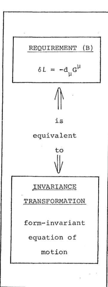
so that requirement (B) is not met, and in general a conservation law does not follow.

To see that requirement (B) is equivalent to the requirement of an invariance transformation, and hence ensures a symmetry transformation, recall the transformed equation of motion

(2.4.20

E<j>,{L' [x')}

=

0 (2.4.21)

Using requirement (B) [equation (2.4.4)j in terms

of

the primed variables, the left-hand side of equation (2.4.21) becomes

Appendix E has a proof of the general identity that

for any G(x,¢,¢l-l •••). Using this, equation (2.4.23) becomes

(2.4.22)

E¢

1 { L 1

[x 1

] }

=

E¢

1 { L [x 1

] }

so that the transformed equation of motion is

E¢

1

{L[x']}

=

0

Clearly, this is of the same functional form as the original equation of motion

Hence the transformation is an invariance transformation, and since this process is reversible, requirement (B)

(2.4.25)

(2.4.26)

(2.4.27)

is equivalent to the assumption of an invariance transformation. Since an invariance transformation must leave the solution

set invariant, requirement (B) ensures the transformation is a symmetry transformation.

Refer to figure (2.3) for a schematic of the relationships between requirement (B) , invariance and symmetry transformations.

Although conventional Noether1_{s theorem is a more}

restrictive formulation than is necessary, i t has enjoyed some success in application. One reason for this is that many physical systems [e.g. linear field systems,

discrete many-body systems] have conservation laws associated with transformations under which requirements (A) and (B)

are met. Another reason could be the ready physical

[image:37.597.69.250.199.678.2]

FIGURE (2.3}

A Schematic of the Relationships Between Requirement (B), Invariance Transformations,and Symmetry Transformations.

REQUIREMENT (B)

oL

=

-d Gll J-l

.

~s

equivalent to

~

INVARIANCE TRANSFORMATION

form-invariant equation of

motion

does not imply

SY!'L"1ETRY

TRANSFORMATION

the use of conventional Noether's theorem on those systems with a scalar Lagrangian density, see appendix B.

A less restrictive method for checking that a transformation leaves the action integral functionally invariant is discussed in the next section.

{2~5) AN ALTERNATIVE APPROACH TO NOETHER'S THEOREM

The problem in applying Noether's theorem of section (2.3) is to check that

oJ

is zero. The technique in the previous section (2.4) has the drawback of being sufficient but not necessary that

oJ.

be zero, and hence of being

more restrictive than necessary. An approach is presented in this section that gives a necessary and sufficient

condition that 6J be zero.

A necessary and sufficient condition that the

funotionaZ variation of the action integral be zero is

that

( {2.5.1)

where

oL _

z:

a a¢111 ••• ila

aL

_o¢

₊

_a

_(Lox

_{11 )}

ill ••• lla axil 1 (2.5.2}

and where

G11

vanishes on the boundary of

v

and

J.

aL

cS<P

+_a-

(Lox11

)Jdx

1Jl ••• 1J _a "1J _ax

which gives, from definition (2.5.2),

8]

=

I

cSLdx

v

(2.5.3)

(2.5.4)

Theri clearly, cSJ is zero if and only if cSL is the divergence of a term that vanishes on the boundary of v, as discussed at equation (2.3.3).

The condition (2.5.1) is related to requirements (A) and (B) as follows:

Recall requirement (A) as expressed in equation (2,4,1) 1

L 1 _[x 1

] dx 1

=

L [x] dx (2.5.5)

Using equation (2.1.5) for the transform of the infinitesimal four-volume dx, this becomes

{L1 _[x1

] - L[x] + L1 [x1]d

11 (ox 11 )}dx

=

0 (2.5.6)

or, to first-order in the variation, and since dx is nonzero,

(2.5.7)

[oL] _ L' [x'] - L[x]

+

L[x)d~(ox~)

requirement (A) becomes, in another form,

[o

L

1

=

o

Requirement (B) is recalled to be

8L-

L'[x]- L[x]

=

d G~

~

Using the definitions (2.5.8) and (2.5.10),

[ 0 L] -

8

L

=

L ' [X ' ] + L [X] dy ( 0 X~) - L ' [X] •

A Taylor expansion gives

(2.5.8)

(2.5.9)

(2.5.10}

(2.5.11)

[oL] -

8L

₌

_I

a 3¢'

~1

d L I

o"''

'I' ll1 •••

~

+

~

ox~

+ _{L [x]d}

(ox~)

a axll ~

•• • ~a

(2. 5 .12)

which is, to first order in the variation,

[oLJ -

8L

=

I

_aL _ _ _

_

3¢~1 _{• • • ~a}

o¢~1

• • •

~

a

+_a

_o "'x~

-(Lox~)

• (2.5.13)

The right-hand side of this equation has been defined as

oL,

so that

This equation, together with the equations (2.5.9} and (2.5.10) for requirements (A) and (B), is the key

to the relationship between these requirements and condition (2.5.1).

Clearly, requirements {A) and (B) are sufficient but not necessary conditions that 'oL be a divergence.

Many authors [e.g. Hill(l951), Dothan (1971), Schroder (1968)] derive condition (2.5.1) as a requirement on the transform-ation that i t leave

J

invariant, but they do so by assuming requirement (A) holds as a property of the Lagrangian,

so that from equation {2.5.14),

oL

= -

"8L

(2.5.15)

That is, under assumption {A), condition {2.5.1) is identical to requirement (B) .

Rosen (1971) has a detailed discussion of the points made here, and Dass (1966b) has a derivation of condition

(2.5.1).

The advantages of this alternative approach to checking that oJ is zero are that i t is both necessary and sufficient, and that i t is easy to check any Lagrangian L for this

property, given a transformation (ox,o¢). The function GP [if i t exists] can be computed directly from equations (2.5.1) and ( 2 . 5. 2) ~

and the corresponding conservation law can be found by substitution into conservation equation (2.3.6):

..

(2.5.17)

If the left-hand side of equation (2.5.16) will not

form a four-divergence, 8] is not zero and Noether's theorem does not apply.

(2.6) GENERALISED NOETHER'S THEOREM

Rosen '(1972, 1974a, .1974b) has generalised Noether's theorem so that a Lagrangian is no longer needed to be able to associate an infinitesimal transformation with a conservation law. Since some equations of motion do not possess Lagrangians, this is quite a useful generalisation.

All that is required is the equation of motion, and the transformation

6¢.

Note that 8x is no longer explicitly required, as will be discussed in section (2.7).

Generalised Noether's theorem states that

i f the

infinitesimal transformation

8¢

is such that

- 6¢

F

=

d Jll - K

ll

holds for general field

variables¢~

where

K(x,¢,¢l1 •••)

is zero for solutions and is linearly independent of

F~

and where

F

=

0

is the equation of motion for the system, then

~¢

is

assoaiated with the conservation equation,

d J11

=

0

11

for solutions.

It will be shown that if a Lagrangian exists for a system, generalised Noether's theorem is

equivalent

to the alternative approach to Noether's theorem in section

(2.5),

i f

K

is identically zero.

Compare equation (2.6.1) with Noether's relation, equation (2.3.4):

The only difference is that K is identically zero in Noether's relation [that is, K is not there].

(2.6.2)

(2.6.3)

Any transformation (ox,~¢) associated through Noether's theorem with a conservation law, must be such that Noether's relation holds if the system has a Lagrangian, and hence must be such that generalised Noether's relation (2.6.1) holds with K identically zero.

To see what generalised Noether's theorem implies for a system with a Lagrangian, in particular to see what

oL -

I

aL

a (3.+.

'I' lll •••

(2.6.4)

Recall the work in section (2.1), in which the right-hand side of equation (2.6.4), as the integrand in

J,

was

rearranged until i t was obtained in the form

(2.6.5)

If generalised Noether's relation (2. 6 .1) is satisfied, substitution for 6¢Eq,(L) in equation (2.6.5) gives

(2.6.6)

where K is zero for solutions and is linearly independent of the equation of motion.

If K were identically zero in the above equation,

condition (2.5.1) of the alternative approach to Noether's theorem would be satisfied, that is,

(2.6.7) where

(2.6.8)

so that the functional variation of the action integral would be zero.

In general, however, K is zero only for solutions, and

oL

is equal to a divergence term plus K, so that

oJ :::::

Jv oLdx

=

Jv

(d Gll

ll

=

J

Kdx 1 v

(2.6.9)

+

K) dx

1 (2.6.10)

(2.6.11)

under the usual assumption that Gll vanishes on the boundary of v. Hence 6J is zero only for solutions to the equation of motion. This is not saying anything new about 6J, since i t is always zero for solutions, under the usual assumption

that~ ••• ,, vanishes, for all a> 0, on the boundary of

Jll t-< a

v. This follows from Hamilton's principle, and also from the form of equation' (2.1.19) .for oJ:

8]

r

, . _ r u,, ... ~l

₊

' " 11,

₊

t:~ .... 1 1 \ t . . : l ••

=

Jv tall L

1T' ~ L) o (jl LUX j Ulj!.C.$\1-J)Uh _f (2.6.12)

=

Jv "&$Ecp(L)dx

(2.6.13)

So generalised Noether's theorem gives a slight gen-eralisation of Noether's theorem if a Lagrangian exists, such that 6J is no longer required to be zero1 but such

that a conservation law still arises from the development of 6J in section (2.1) 1 as follows: recall the result of

section (2.1) as expressed in equation (2.6.5),

(2.6.14)

8L

= -

d G~

+

K

~

where K is zero for solutions and is linearly independent

(2.6.15)

of.the equation of motion. Equations (2.6.14) and (2.6.15) yield the conservation law

d J~

-~

=

0

for solutions, even though 8] is not zero.

Howeve~, as Rosen [(1974a), fourth footnote] points out, this slight generalisation of Noether's theorem to include K which is zero only tor solutions does not

(2.6.16)

appear to be of much practical use. In most practicaZ cases~ K is identicaZZy zero and generaZised Noether's theorem is equivaZent to Noether's theorem whenever a Lagrangian exists

for the system.

If a Lagrangia~ does exist for a system, Noether's theorem is a more powerful approach to conservation laws than generalised Noether's theorem, since i t allows the prediction of conservation laws from properties of the

Lagrangian. For example, as in appendix C, if a Lagrangian is not explicitly dependent on the z-coordinate, i t

immediately follows from Noether's theorem [the alternative approach] that the z-component of linear momentum is

with integra-differential equations of motion.

The property of K that i t be linearly independent of the equation of motion is necessary to prevent the association of 8~ with J~ from being ambiguous. As is mentioned by Rosen [(1974a), second footnote], if K was allowed to depend linearly on the equation of motion, any arbitrary infinitesimal transformation could be

trivially associated with a given conservation equation.

This is apparent from generalised Noether's relation (2.6.1):

=

d J~ - K

~ (2.6.17)

If a variation 8~ exists such that generalised Noether's relation holds, take an arbitrary variation 62~. Then from equation (2.6.17),

(2.6.18)

and if K is allowed .to depend linearly on E~(L), this

equation can be put into the form of generalised Noether's relation:

where

In such a way, any arbitrary infinitesimal transformation can be associated with J~ unless K is restricted to be

(2.6.19).

linearly independent of the equation of motion. Candotti, Palmieri and Vitale (1972) in their

treatment of Noether's theorem have as the condition on

oL,

(2.6.21)

where f may be linearly dependent on the equation of motion. Comparing this condition to generalised Noether's condition

(2.6.6), i t is apparent that f equals K. Not surprisingly, these authors conclude that any infinitesimal transformation can be associated through Noether's theorem with any existing conservation law. Their conclusion is a consequence of

the ambiguity inherent in their condition (2.6.21).

It should be noted that in any use of conventional or generalised Noether's theorem, the requirements (A) and

(B) in section (2.4), condition (2.5.1) or condition

(2.6.1) must be shown to hold for general field variables

¢.

Any unwitting use of the equation of motion to help prove that these requirements are met, will succeed in associating any transformation with any existing conservation law. For example,condition (2.6.1) would hold trivially, since both sides are always zero for solutions if J~ is a conserved vector, enabling any choice of variation

6¢.

(2.7) THE NOETHER FAMILY OF TRANSFORMATIONS

Noether's theorem, and in understanding why 6x does not explicitly appear in generalised Noether's theorem.

The transformation associated with a conservation law in generalised Noether's theorem is characterised by 6¢. Since [equation (2.1.11)]

'

there is a set of values of (6x,6¢) with the same value

of o¢> and hence associated with the same conserved

vector J~ and the same K> through generalised Noether's

theorem. Candotti, Palmieri and Vitale (1970) refer to

this set {(6x,6¢)} as a Noether family.

Rosen (1972) shows by a formal construction that

every Noether family contains a transformation (6x,6¢)

such that the Lagrangian [if i t exists] transforms as

a scalar density> which is condition (A) of conventional

Noether's theorem, that is,

(2.7.1)

[6L]

=

0 (2.7.2)

as in equation (2.5.9). A proof of this follows. Recall equation (2.5.14) ₁

6L

=

[6L] - 8L

and equation (2.6.6) for 6L when generalised Noether's relation (2.6.1) holds,

(2.7.4)

Combine equations (2.7.3) and (2.7.4} to get

(2.7.5)

Without loss of generality, divide

5L

into a divergence and a nondivergence term:

{2.7.6)

Substitute ~his into equation (2.7.5) to get

[ o

L

l

(2.7.7)

Let a Noether family be associated with the conservation law,

0

for solutions. Take one member

(o1x,o1¢)

of this family, and formally construct another member

(82x,o2¢}

in terms of the first member, as in Rosen (1972}:

I

{2.7.8)

,

Note that o

2

x~ is dependent on ¢ in this construction. This does not invalidate the result, even though ox has been assumed to be dependent only on x in this chapter.

If the values in equations (2.7.9) are substituted into equation (2.7.7) for [62L],

[62 L]

=

d~[TI~(L)iS¢

+

Lo2x~- J~

+

o2LPJ

everything cancels to give

and the proof is complete.

If, as is usuaily the case [see appendix F], K is identically zero,

that is, condition (B) of conventional Noether's theorem

(2.7.10)

(2.7.11)

(2.7.12)

is also met. Hence,

i f

K

is identicaZZy

zero~

requirements

(A) and

(B)

of conventional Noether's theorem wiZZ be met

Clearly, if K is identically zero, condition (2.5.1) of the alternative approach to Noether's theorem is met by all members of the Noether family. This is proved at equation (2.6.7).

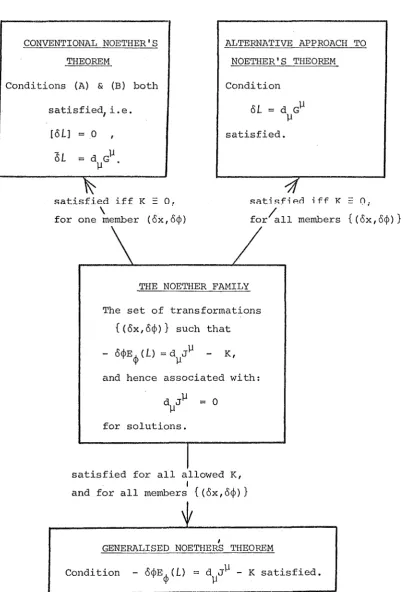
Figure (2.4) summarises in schematic form these

relationships between the different approaches to Noether's theorem, in terms of the Noether family.

One feature of Noether's ~heorem has been brought into the open by generalised Noether's theorem and the concept of a Noether family of transformations. This is the irrelevance of the coordinate transformation ox to the existence of-a conservation law, except as i t

affects

8¢.

Changing ox while keeping

8¢

the same will not change the associated conservation law [if i t exists], although i t will change the values of

[oL]

and

8L,

as seen earlier in this section.

The irrelevance of ox corresponds to the equivalence of the active and passive views of a coordinate transform-ation [Saletan and Cromer (1971)]. For example, a translation can be viewed passively as a shifting of the coordinate

axes, while the field variables remain stationary. The variation would then be

ox~

=

8~ [infinitesimal]' o¢

=

0

and hence

(2.7.13)

FIGURE (2.4)

Schematic of Relationships Between Different Approaches to Noether•s Theorem and the Noether Family of Transformations

CONVENTIONAL NOETHER'S THEOREM

ALTERNATIVE APPROACH TO NOETHER'S THEOREM

Conditions (A) & (B) both Condition satisfied, i.e.

roLJ

=

o

satisfied.

6L

satisfied iff K ~ 0. RatisfiAd iff K ~ 01

for/all members {(ox,o¢)}

\ .

for one member (ox,o¢)

THE NOETHER FAMILY

The set of transformations {(ox,o¢)} such that - o¢E¢(L)=d

1

_/J.l

K, and hence associated with:

for solutions.

satisfied for all allowed K,

I

and for all members {(ox,o¢)}

I

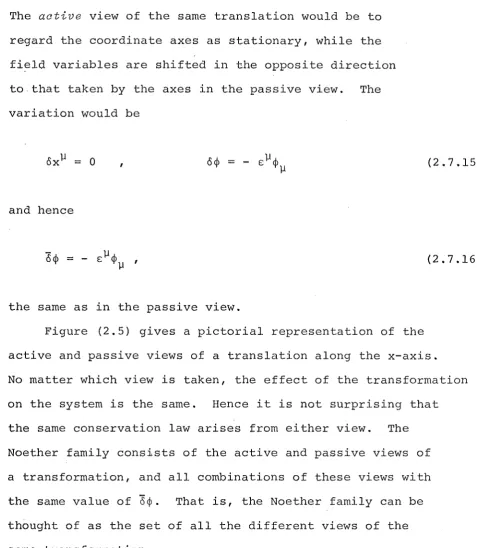
[image:53.597.77.480.192.784.2]

The active view of the same translation would be to regard the coordinate axes as stationary, while the

fi~ld variables are shifted in the opposite direction

to that taken by the axes in the passive view. The variation would be

ox~

=

0

and hence

the same as in the passive view.

(2.7.15)

(2.7.16)

Figure (2.5) gives a pictorial representation of the active and passive views of a translation along the x-axis. No matter which view is taken, the effect of the transformation on the system is the same. Hence i t is not surprising that the same conservation law arises from either view. The Noether family consists of the active and passive views of a transformation, and all combinations of these views with the same value of

8¢.

That is, the Noether family can be thought of as the set of all the different views of the same transformation.

[image:54.595.58.536.72.621.2]

FIGURE (2.5)

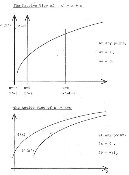
The Active and Passive Views of an x-Translation.

The Passive View of

~'(x') ~(x)

I

x=-8 x'=O

x=O x'=8

x'

=

x

+ 8

x=k x'=k+8

The Active View of x' = x+8

at ox

0~

any point, =

=

X

8 ,

o.

point, 0

-8~ •

[image:55.595.66.508.178.773.2]

families are a useful labelling system for their

associated conservation laws, and can be used to ide~tify a conservation law as follows:

For example, if a conservation law was found to be associated via Noether's theorem with the variation

where 8 is an infinitesimal parameter, the law would be_

identified as expressing conservation of energy. This follows from the work in app~ndices B and C, which show that conservation of energy is associated with such a variation.

Note that in the passive view of transformation (2.7.17),

ot = 81 OX~ = 0 for X~ ~ t, o¢ = 0

(2.7.17)

(2.7.18)

CHAPTER III

(3.1) BACKGROUND

The Korteweg-de Vries [KdV] .e.quation has been the subject of much research interest in the last 18 years. It was originally derived by Korteweg and de Vries (1895) for the evolution of long water waves down a rectangular canal, in the form

in one space dimension and time, where n is the surface elevation above the equilibrium level ~, a is a small arbfrrary constant related to the uniform motion of the liquid, g is the gravitational constant and

(J

=

with sur

~3

3

T ~

pg

I

tension T and density p.

Despite the general suitability of the KdV equation

(3.1.1}

(i) ion-acoustic waves in plasma, by Washimi and Taniuti (1966), and Tappert (1972).

(ii) the anharmonic lattice, a one-dimensional

lattice of equal masses coupled by nonlinear springs, also known as the Fermi-Pasta-Ulam problem (1955), by Zabusky (1967, 1973).

(iii) longitudinal dispersive waves in elastic rods, by Nariboli and Sedov (1970).

(iv) pressure waves in a liquid-gas bubble mixture, by Wijngaarden (1968).

(v) The axial component of velocity in a rotating fluid flow down a tube, by Leibovich (1970).

(vi) thermally excited phonon packets in low-temperature nonlinear crystals, by Tappert and Varma (1970). A large class of nonlinear Galilean-invariant systems, under the assumptions of weak nonlinearity and long

wavelength, have been shown to reduce to the KdV equation in the work of Su and Gardner (1969) and of Leibovich and Seebass (1974). A general class of nonlinear systems has been reduced by a perturbation method t6 the KdV equation by Taniuti and Wei (1968), and Zielke (1974) has shown that a wide class of nonlinear partial differential equations derivable from a variational principle also reduces to the KdV equation.

However~

it has been the properties of the

KdV

equation

and its solutions that have primarily motivated much of

be noticed was the existence of solitary wave solutions which emerge from a collision with the

same

shapes and velocities as before i t [Zabusky and Rruskal (1965)]. An

exaat method

for solving the KdV equation by means of a linear scattering problem was published by Gardner, Greene, Kruskal and Miura (1967). The existence of an

infinite

number of aonserved densities)

each of the form of a

polynomial in the field variable

n

and its x-derivatives, was proved in a publication by Miura, Gardner and Kruskal (1968). Wahlquist and Estabrook (1973, 1975) discovered the

Backlund transformation

for the KdV equation, which

' '

maps solutions to solutions.

These properties of the KdV equation and its solutions are all inter-related. A brief resume of them follows in sections {3.2} to (3.5). The remainder of this chapter investigates what light can be shed on the infinite number of polynomial conserved densities by the techniques of Noether's theorem. This includes work done by Steudel

(1975b), associating an infinitesimal extended Backlund

transformation with the infinite set of densi , and original work identifying each density as an energy or a momentum

density.

(3.2) THE INVERSE SPECTRAL METHOD OF SOLUTION

spectral method

[I.S.M.] for solving exactly the initial-value problem. That is, ~iven. a solution u of the KdV equation at a time

t

0 , find the solution after a time

tr

has elapsed. This problem was previously only approximately solvable for the KdV equation by numerical methods

[e.g., Zabusky and Kruskal (1965)], and the only exact solutions known were the solitary and cnoidal waves

[Korteweg and de Vries (1895)]. The I.S.M. has subsequently been applied to other nonlinear equations with some

success, and to a broad class of nonlinear equations by Ablowitz, Kaup, Newell and Segur (1973).

The most convenient form of the KdV equation for applying the I.S.M. is

ut - 6uux

+

u _XXX = 0 {3.2.1)

The scale transformation

- n -

a

u

=

-

I

2 3

t '

₌

1

[:art

2 I

x'

=

(J

-!.!

X

'

to the.KdV equation is to regard u(x,t) as the potential in the time-independent one-dimensional Schrodinger

scattering equation,

1)! (x,t) - [u(x,t) - A.(t)]1)i(x,t)

=

0 XX

The time coordinate in equation (3.2.1) appears only

(3.2.2)

parametrically in equation (3.2.2). The direct scattering

problem in quantum mechanics is to be given the potential

u (x) , and to find the asymptotic behaviour of 1)! (x) . at

x

=

+

oo, and the bound state energy levels and normalisation constants, otherwise known as the scattering data. The

techniques for solving this problem are well-known [see, for example Schiff (1968)].

The inverse scattering problem is to find the

potential u(x) given the scattering data. The technique will be outlined here in the usual quantum mechanical context, that is, with t fixed.

The key to the use of the I.S.M. to solve the KdV equation is that i f the potential u(x,t) is allowed to evolve in the

parameter t according to the KdV equation~ the discrete

eigenvalues Am do not change~ and the other scattering

data change in a simple way with the parameter t. The Schrodinger equation (3.2.2) has a set of continuous eigenvalues

and discrete eigenvalues

(3.2.4)

The eigenfunctions of the discrete eigenvalues are normalised:

(3.2.5)

and for the continuous eigenvalue's, the scattering problem is set as

1Ji c:: exp(-ikx) +bexp(ikx), for x-+

oo,

(3.2.6) 1Ji c:: a exp (-ikx), for x -+ -oo ₁

and i t can be shown that

lal

2

+

lbl

2 = 1

The scattering data are then the quantities km' em and b(k}. The key discovery by Gardner, Greene, Kruskal and

Miura {1967} was that the scattering data depend in a very simple way on the parameter t if u(x,t} is required to be a solution of the KdV equation {3.2.1). Their work

showed that

Am (t)

=

Am (0)

,

a(k,t)

=

a{k,O) _I

b(k,t)

₌

b{k,O)exp(8ik3t) _I en (t)

=

cn(O}exp(4k~t),

where Am(O), b(k,O) and cn(O) are determined from the initial data for the KdV equation, u(x,O), by the

direct

saattering problem.

It is assumed that k is independent of t, to find a and b.

The

inverse scattering problem

can then be solved for A(t), b(k,t) and cn{t) to find [exactly] u(x,t} at any time t. This problem has been studied by Gel'fand and Levitan (1955), Kay and Moses (1956), and Levinson (1953). They show that the solution is

u = - 2 d dx

K(x,x) , (3.2.8)

where K satisfies the Gel'fand-Levitan integral equation

K(x,y) + B(x+y) +

Joo

B(y+z)K(x,z}dz = 0 X

The kernel B is given in terms of the scattering data:

Note that dependence on the parameter t in B and K has been suppressed in these equations.

(3.2.9)

(3.2.10:

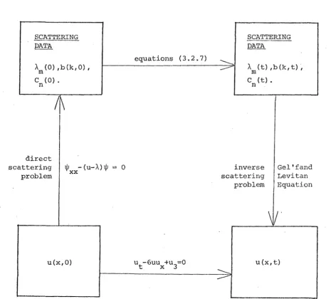
To summarise, the !.S.M. for solving the KdV equation is as follows: beginning with an initial solution to the KdV equation, u(x,O), solve the direct scattering problem

new scattering data Am(t), b(k,t) and cn(t) into

equation (3.2.10) to find B(x;t), and solve the [linear] Gel'fand-Levitan integral equation (3.2.9) to find K(x,x) and hence u(x,t).

The I.S.M. for solving the KdV equation is shown diagrammatically in figure (3.1).

Although explicit solutions·u(x,t) cannot be obtained in general, exact solutions can be given for the cases when b(k,O) is zero [no reflection of ~ from the potential u], as in Gardner, Greene, Kruskal and Miura (1974). The main simplification achieved is that all equations to be solved are linear.

The form of B in equation (3.2.10) suggests a link with the Fourier transform technique for solving linear equations. Ablowitz, Kaup, Newell and Segur (1974) show that the I.S.M. does reduce to the Fourier technique on linearisation of the equations of motion, and that the

I.S.M. may be regarded as a generalisation to nonlinear

systems of the Fourier transform method.

(3.3) SOLITON SOLUTIONS

A soliton is a particular type of solitary wave or

localised travelling wave. The working definition of Scott, Chu and McLaughlin (1973) will be adopted, that a soliton is a solitary wave solution of a wave equation which asymptotically

preserves its shape and velocity upon collision with other