Division VI
DESIGN OPTIMISATION OF STACK USING TIME
DOMAIN SEISMIC ANALYSIS
John Hadfield1, Ming Tan2, Ryan Gumley3 and Yasuo Nitta4
1
Principal Engineer, Mott MacDonald Ltd, United Kingdom
2 Discipline Lead for Advanced Analysis, Mott MacDonald Ltd, United Kingdom
3 Graduate Engineer, Mott MacDonald Ltd, United Kingdom
4
General Manager, Shimizu Corporation, Japan
ABSTRACT
This paper presents an alternative approach to the more conventional response spectrum method for the design of a stack structure, ie. by using time domain seismic analysis and with the design undertaken at each individual time step.
The response spectrum approach is often conservative, the sign of the results is lost during modal combination and the actual response in time is not quantifiable. Subsequent design that uses the maximum of all component stresses is therefore inaccurate, and the loss of detailed information makes the design of construction details challenging. Using time history analysis, the results for the stack structure are obtained with the correct signs at every time step for the duration of the earthquake.
Comparison of results, in terms of utilisation ratios (UR) are presented with benefit of the time history approach quantified. In summary, the time history approach gives a better and more comprehensive representation of structural behaviour and a more economical design, and the results are easily adaptable for study beyond the design basis.
INTRODUCTION
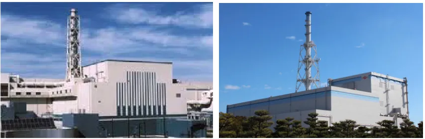
The objective of this paper is to consider the design optimisation of a stack structure using time domain seismic analysis. With similar configuration of the stack structures of a boiling water reactor (see Figure 1), the stack consists of a surrounding lattice frame support tower of rolled steel sections and enclosed chimney of thin shell construction, located on the roof of a reactor building. Due to the amplification of the reactor structure and roof responses, the accelerations to the stack substructure are generally very high.
Conventional seismic analysis would make use of floor response spectra to generate seismic forces. The response spectrum approach is generally conservative, the sign of the results is lost during modal combination and the actual response in time is not quantifiable. Subsequent design uses the maximum of all component stresses and is therefore often grossly conservative (or just inaccurate), and leads to complex and challenging construction details.
Figure 1: Stack Structures at Kashiwazaki-Kariwa & Tokai Daini NPPs (photos extracted from www.alamy.com)
As shown in Figure 1 above, the stack structure considered in this paper is typical of a boiling water reactor main stack, which consists of two main parts, the lattice frame and the chimney. The lattice frame (tubular hollow steel sections) provides lateral support to the chimney (stainless steel thin plate). Details of the corresponding Finite Element (FE) model are provided in the Geometry & Loading section below. This configuration of stack structure is specifically chosen for this study as it consists of steel elements which are designed using forces & moments and stack shells which are designed using stresses.
The stack structure is subject to static dead vertical gravitational (1g) loading and also dynamic earthquake loading in the 3 spatial directions, ie. North-South (NS), East-West (EW) and Up Down (UD).
Three methods are considered for the implementation of the seismic loading and extraction of results for design in this paper, as follows:
• Method 1: The response spectrum analysis method is used for the stack. This is a conventional
method for seismic analysis and combines the modal response at each frequency due to the earthquake acceleration into a single positive value for each of the member results of the stack.
• Method 2: The time history analysis method is used for the stack, considering full integration within the time domain. This method produces results at each time step during the earthquake loading but for design purposes the maximum values (ie. not necessarily concurrent) are chosen for code checking.
• Method 3: This method uses time history analysis as per Method 2 but for design purposes the
concurrent values at each time step are used for code checking, ie. the design is performed multiple times (at every time step) and the most onerous value (ie. maximum UR) is noted from all the time steps.
The results of each method are summarised in the respective sections below for Method 1, Method 2 and Method 3.
GEOMETRY & LOADING
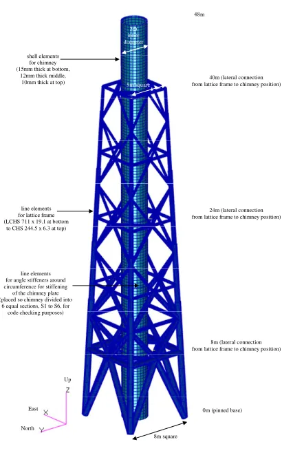
The geometry of the stack is incorporated into the FE model as illustrated in Figure 2. The FE program NASTRAN (MSC, 2013) is used for the modelling and analysis. The analysis is linear elastic. The lattice frame tubular hollow steel sections are modelled with 2-noded line elements (CBAR) and the chimney stainless steel thin plates are modelled with 4-noded shell elements (CQUAD4).
The input loading is the static dead vertical gravitational (1g) loading and the dynamic earthquake loading in the 3 spatial directions (NS, EW, UD).
The static dead vertical gravitational (1g) loading is applied to the model (via grav command using
9.81ms-2) such that the model mass and gravitational
acceleration produce the applied force vector. This static dead load is unfactored and is notated as 1.0D.
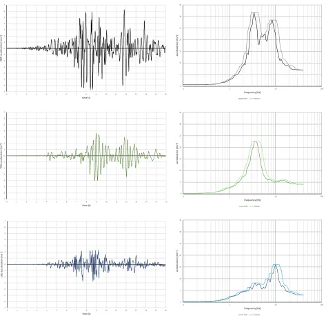
The earthquake loading is defined by the 3 acceleration time histories shown in Figure 3 (for XEW, YNS, ZUD). It can be seen that XEW horizontal direction is the most onerous with a duration of 16s and a peak of
~7ms-2 or 0.7g, typical of acceleration on the top of a
reactor building roof. The time step size of the input data is 0.005s (ie. 16s/0.005s = 3200 data points).
For the time history seismic analysis (Method 2 & Method 3), the acceleration time histories are applied directly to the base of the model. The equation of motion is solved by direct integration in the time domain. A target 4% damping value is used. Since the results require the static loading to also be present, the static load is applied as an initial condition in the time history analysis and kept constant for the duration of the time history load.
For the response spectrum analysis (Method 1), the equivalent acceleration floor response spectra (at 4% damping) are generated from the acceleration time histories. These are shown for each direction in Figure 3 below. The response spectra curves are used to factor each mode's results (from an undamped eigenvalue solution for the equation of motion) and then the modes are combined to give the analysis result, denoted as E (all results in absolute magnitude due to loss of sign in modal and spatial combination). The static load is included at the post processing stage, ie. results 1.0D+E and also (due to oscillating dynamic load) 1.0D-E created.
To account for the uncertainty in seismic data, the floor response spectra are smoothed and peak broadened by ~15% as seen in Figure 3. The smoothing and peak broadening are performed to widen the band of frequencies that see a higher acceleration, thus accounting for uncertainty / possible non-conservatism in the input seismic data. This is a common approach within response spectrum analysis. A comparative technique (as per section 6.3.2 (b) of ASCE 4-16 [4]) is performed for the time history analyses, which adjusts the time step by -/+15%, ie. additional time history analysis is performed with the time step at 0.00425s (-15% on time, frequency increased) and with the time step at 0.00575s (+15% on time, frequency decreased). Note that the results account for these additional +/-15% analyses. The results of the 3 methods are summarised in the following sections.
48m
0m (pinned base) 8m (lateral connection from lattice frame to chimney position)
24m (lateral connection from lattice frame to chimney position)
40m (lateral connection from lattice frame to chimney position)
Up
East
North shell elements
for chimney (15mm thick at bottom,
12mm thick middle, 10mm thick at top)
line elements for lattice frame (LCHS 711 x 19.1 at bottom
to CHS 244.5 x 6.3 at top)
line elements for angle stiffeners around circumference for stiffening of the chimney plate (placed so chimney divided into
6 equal sections, S1 to S6, for code checking purposes)
8m square 5m square
3m inner diameter
-7 -6 -5 -4 -3 -2 -1 0 1 2 3 4 5 6 7
0 1 2 3 4 5 6 7 8 9 10 11 12 13 14 15 16
X E W a c c e le ra ti o n ( m s -2) time (s) 0 5 10 15 20 25 30 35
0 1 10 100
a cc e le ra ti o n ( m s -2) frequency (Hz) XEW XEWsm -7 -6 -5 -4 -3 -2 -1 0 1 2 3 4 5 6 7
0 1 2 3 4 5 6 7 8 9 10 11 12 13 14 15 16
Y N S a c c e le ra ti o n ( m s -2) time (s) 0 5 10 15 20 25 30 35
0 1 10 100
a cc e le ra ti o n ( m s -2) frequency (Hz) YNS YNSsm -7 -6 -5 -4 -3 -2 -1 0 1 2 3 4 5 6 7
0 1 2 3 4 5 6 7 8 9 10 11 12 13 14 15 16
Z U D a c c e le ra ti o n ( m s -2) time (s) 0 5 10 15 20 25 30 35
0 1 10 100
a c ce le ra ti o n ( m s -2) frequency (Hz) ZUD ZUDsm
METHOD 1: RESPONSE SPECTRUM ANALYSIS, RESULTS
The results for Method 1 (similar tables for Method 2 & Method 3) are first tabulated for the lattice frame. A few selected elements are chosen for illustration purposes. The maximum (max.) utilisation ratio (UR) is shown and is due to the interaction of the line element reactions, ie. the axial force P and the bending moments Mx & My. The corresponding allowables are Pnc (for axial compression, -ve, which governs) and Mcx & Mcy. As per the AISC N690-12 code [1] (where the value of P/Pnc is > 0.2), the UR is calculated as |P|/Pnc + 8/9*(|Mx|/Mcx+|My|/Mcy).
Table 1a: Method 1 (Response Spectra) Lattice Frame Results
Line
Element Description
load for max. UR
P Pnc (kN)
Mx Mcx (kNm)
My Mcy (kNm)
max. UR
5 LCHS 711 x 19.1
column near base 1.0D-E
-4775 11779
-218 2651
-197
2651 0.54
11 LCHS 610 x 17.5
column at mid-height 1.0D-E
-2847 9178
-173 1782
-112
1782 0.45
12 CHS 508 x 10
column at mid-height 1.0D-E
-2844 4478
-94 693
-80
693 0.86
16 CHS 508 x 10
column at ¾ height 1.0D-E
-1516 4478
-93 693
-72
693 0.55
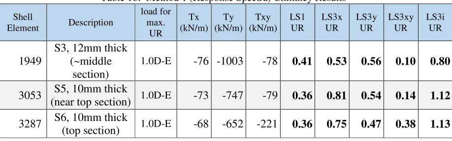
The next table is for the code check of the chimney. Again a few elements are selected. The code checks consider the LS1 plastic limit state (using the Von Mises equivalent stress – from all the component stresses), the LS3x buckling limit state (using the Tx horizontal / circumferential stress component), the LS3y buckling limits state (using the Ty vertical / meridional stress component), the LS3xy buckling limit state (using the Txy shear stress component) and the LS3i buckling limit state (considering the interaction of all the component stresses). Moments are negligible so only the Tx, Ty, Txy shell forces are used to derive the corresponding stresses. BS EN 1990:2002 [2] is used to derive the allowable LS1 and LS3 stresses (for each of the chimney sections, S1 to S6). Note that for the LS3 buckling checks, only the -ve (compressive / buckling) stresses are appropriate.
Table 1b: Method 1 (Response Spectra) Chimney Results
Shell
Element Description
load for max.
UR
Tx (kN/m)
Ty (kN/m)
Txy (kN/m)
LS1 UR
LS3x UR
LS3y UR
LS3xy UR
LS3i UR
1949
S3, 12mm thick (~middle
section)
1.0D-E -76 -1003 -78 0.41 0.53 0.56 0.10 0.80
3053 S5, 10mm thick
(near top section) 1.0D-E -73 -747 -79 0.36 0.81 0.54 0.14 1.12
3287 S6, 10mm thick
METHOD 2: TIME HISTORY ANALYSIS, USE MAXIMUMS, RESULTS
The table shows the UR values for the lattice frame, using the maximum (accounting for sign) values. Since maximum values are used, values are not necessarily concurrent (eg. for My).
Table 2a: Method 2 (Time History, Maximums) Lattice Frame Results
Line
Element Description
time for max. P Mx My
max. P Pnc (kN)
max. Mx Mcx (kNm)
max. My Mcy (kNm)
max. UR
5 LCHS 711 x 19.1
column near base
12.650s 12.650s 9.625s
-5115 11779
231 2651
-205
2651 0.58
11 LCHS 610 x 17.5
column at mid-height
12.650s 12.650s 9.475s
-2952 9178
-177 1782
135
1782 0.48
12 CHS 508 x 10
column at mid-height
12.650s 12.650s 9.325s
-2948 4478
-99 693
-88
693 0.90
16 CHS 508 x 10
column at ¾ height
12.650s 12.500s 9.325s
-1494 4478
84 693
-75
693 0.54
The table shows the UR values for the chimney, using the maximum (ie. most -ve for buckling) force values (from which the stresses are derived for the code check). Since maximum values are used, force (stress) values are not necessarily concurrent. Note, for UR values that correspond to Method 3 (ie. rely
on single stress components) the values are displayed in blue font.
Table 2b: Method 2 (Time History, Maximums) Chimney Results
Shell
Element Description
time for max. Tx
(kN/m)
Ty (kN/m)
Txy (kN/m)
LS1 UR
LS3x UR
LS3y UR
LS3xy UR
LS3i UR
1949 S3, 12mm thick
(~middle section)
Tx Ty Txy
12.625s 9.475s 12.775s
-52 -947 -44 0.39 0.36 0.53 0.05 0.59
3053 S5, 10mm thick
(near top section)
Tx Ty Txy
8.725s 9.475s 12.775s
-78 -500 -58 0.24 0.86 0.36 0.10 1.00
3287 S6, 10mm thick
(top section)
Tx Ty Txy
8.725s 9.475s 8.725s
METHOD 3: TIME HISTORY ANALYSIS, EVERY TIME STEP, RESULTS
The table shows the UR values for the lattice frame, showing the concurrent values at the time at which the max. UR occurs.
Table 3a: Method 3 (Time History, Every Time Step) Lattice Frame Results
Line
Element Description
time for max. UR
P Pnc (kN)
Mx Mcx (kNm)
My Mcy (kNm)
max. UR
5 LCHS 711 x 19.1
column near base 12.650s
-5115 11779
231 2651
1
2651 0.51
11 LCHS 610 x 17.5
column at mid-height 12.650s
-2952 9178
-177 1782
-5
1782 0.41
12 CHS 508 x 10
column at mid-height 12.650s
-2948 4478
-99 693
-3
693 0.79
16 CHS 508 x 10
column at ¾ height 8.725s
-1292 4478
-73 693
-51
693 0.45
The table shows the UR values for the chimney, showing the concurrent values at the time at which the
max. UR occurs (considering the various URs, as shown in bold for relevant row). Note, for UR values
that correspond to Method 2 (ie. rely on single stress components) the values are displayed in blue font.
Table 3b: Method 3 (Time History, Every Time Step) Chimney Results
Shell
Element Description Time (s)
Tx (kN/m)
Ty (kN/m)
Txy (kN/m)
LS1 UR
LS3x UR
LS3y UR
LS3xy UR
LS3i UR
1949 S3, 12mm thick
(~middle section)
LS1 9.475s 3 -947 -3 0.40 - 0.53 0.00 0.32
LS3x 12.625s -52 -323 44 0.13 0.36 0.18 - 0.31
LS3y 9.475s 3 -947 -3 0.40 - 0.53 0.00 0.32
LS3xy 12.775s 46 197 -44 0.08 - - 0.05 0.00
LS3i 9.475s 3 -947 -3 0.40 - 0.53 0.00 0.32
3053 S5, 10mm thick
(near top section)
LS1 9.325s -73 515 26 0.28 0.80 - - 0.75
LS3x 8.725s -78 343 44 0.20 0.86 - - 0.82
LS3y 9.475s 64 -500 -20 0.27 - 0.36 0.04 0.17
LS3xy 12.775s 39 136 -58 0.08 - - 0.10 0.01
LS3i 8.725s -78 343 44 0.20 0.86 - - 0.82
3287 S6, 10mm thick
(top section)
LS1 9.325s -63 458 -111 0.26 0.69 - 0.19 0.67
LS3x 8.725s -70 303 -176 0.23 0.77 - 0.30 0.82
LS3y 9.475s 55 -445 86 0.25 - 0.32 - 0.14
LS3xy 8.725s -70 303 -176 0.23 0.77 - 0.30 0.82
DISCUSSIONS OF RESULTS Lattice Frame
A response spectrum analysis, Method 1, is considered for the seismic analysis of the stack and the results for the lattice frame (line elements) are extracted and code checked (see Table 1a). This method is often conservative in that all modes are combined together with the actual point of occurrence in time not being known.
A time history analysis, considering the maximum values for design, Method 2, is performed as an alternative (see Table 2a). However, since the maximums are used, and not always the concurrent values, this method suffers from the same inherent conservatism as Method 1 – hence for the lattice frame the Method 2 URs are similar (yet generally slightly greater) to Method 1. Method 3 also performs the time history analysis but code checks every time step and so the forces and moments considered are all concurrent (Table 3a). Thus there is no conservatism in the calculations for Method 3. The lattice frame URs are seen to be lower for Method 3 than for the other methods, being on average ~16% lower than Method 2 which is significant for design.
The graphs in Figures 4 (for line element 12) show the variation of the line element reactions and UR with time and illustrate the fact that the max. My value does not occur at the same time as the P and Mx values and hence Method 3 removes the conservatism of considering non-concurrent values for design.
Chimney
The response spectrum analysis Method 1 results are shown to be conservative for the shell stresses with the overall URs for the chimney being highest, with some over utilisations occurring for the LS3i UR checks (max. UR of 1.13, Table 1b). A very clear disadvantage of this method is that when doing stress design, all the component stresses of the stress tensor are the same sign and so derived equivalent stresses are inaccurate. Permutations of +/- component stresses in the stress tensor could be considered but still this does not account for concurrent values and so is still potentially conservative.
-3000 -2000 -1000 0 1000 2000 3000
0.0 1.6 3.2 4.8 6.4 8.0 9.6 11.2 12.8 14.4 16.0
P ( k N ) li n e e le m e n t 1 2 e n d i
time (s )
-50 -40 -30 -20 -10 0 10 20 30 40 50
0.0 1.6 3.2 4.8 6.4 8.0 9.6 11.2 12.8 14.4 16.0
Tx ( kN /m ) sh e ll e le m e n t 1 9 4 9 time (s) -100 -80 -60 -40 -20 0 20 40 60 80 100
0.0 1.6 3.2 4.8 6.4 8.0 9.6 11.2 12.8 14.4 16.0
M x ( k N m ) li n e e le m e n t 1 2 e n d i time (s) -900 -720 -540 -360 -180 0 180 360 540 720 900
0.0 1.6 3.2 4.8 6.4 8.0 9.6 11.2 12.8 14.4 16.0
T y (k N /m ) sh e ll e le m e n t 1 9 4 9 time (s) -100 -80 -60 -40 -20 0 20 40 60 80 100
0.0 1.6 3.2 4.8 6.4 8.0 9.6 11.2 12.8 14.4 16.0
M y ( k N m ) li n e e le m e n t 1 2 e n d i time (s) -50 -40 -30 -20 -10 0 10 20 30 40 50
0.0 1.6 3.2 4.8 6.4 8.0 9.6 11.2 12.8 14.4 16.0
Tx y (k N /m ) sh e ll e le m e n t 1 9 4 9 time (s) 0.0 0.1 0.2 0.3 0.4 0.5 0.6 0.7 0.8 0.9 1.0
0.0 1.6 3.2 4.8 6.4 8.0 9.6 11.2 12.8 14.4 16.0
U R l in e e le m e n t 1 2 e n d i time (s) 0.0 0.1 0.2 0.3 0.4 0.5 0.6 0.7 0.8 0.9 1.0
0.0 1.6 3.2 4.8 6.4 8.0 9.6 11.2 12.8 14.4 16.0
LS 1 U R s h e ll e le m e n t 1 9 4 9 time (s)
Figure 4: Stack Results Through Time
lattice frame P
lattice frame Mx
lattice frame My
lattice frame UR
chimney Tx
chimney Ty
chimney Txy
CONCLUSION
In conclusion, Method 3, where a time domain analysis is performed and code checks are performed every time step, provides an accurate solution and the removal of potential conservative (and non-conservative) values. Computational effort is required to perform checks at each point of the time history, but a simple algorithm is required to loop through the analysis results and repeat the calculation which is required for code checking for whichever method is used.
In some cases, significant reduction in URs are achieved thus leading to an optimum design where section sizes are not increased on the basis of conservative analysis results.
Method 3 also provides accurate and specific information on the behaviour of the structure throughout the duration of the seismic event, not just in terms of the applied forces, moments and derived stresses but also in terms of UR with time.
One of the disadvantages of time history analysis, unlike response spectrum analysis with peak broadened spectra, is accounting for uncertainty in the time history input data. However, running additional analyses with adjustment of the time step of the input time history can account for such uncertainty in a time history analysis.
Furthermore, as well as the time domain analysis being more accurate and informative with respect to design, for consideration of non-linearities, the time domain analysis (full integration) is essential since response spectrum analysis only works for linear scenario.
Based on the results of this work, further work evaluating cliff edge effect due to seismic of the stack structure using fragility analysis have been undertaken (A Andonov et al, 2017).
ACKNOWLEDGEMENTS
The work cannot be completed without the support from Hirokuni Ishikagi-san of Hitachi-GE, of which we are extremely grateful.
REFERENCES
AISC, “ANSI / AISC N690-12 Specification for Safety-Related Steel Structures for Nuclear Facilities”, 31
January 2012
Eurocode, “BS EN 1993-1-6 + UK NA: Eurocode 3: Design of steel structures - Part 1-6: Strength and
stability of shell structures”, British Standards Institution, 2007.
MSC, “NASTRAN User Manual, Version 2013.0.0-CL199358”, MSC, 2013.
ASCE, “ASCE / SEI 4-16 – Seismic Analysis of Safety-Related Nuclear Structures”, 2017.
Andonov A., Tan M. and Y Nitta (2017), “Cliff-edge Seismic Evaluation of Stack Structure Using