Some Properties on the Error Sum Function of Alternating Sylvester Series

(1)

Some Properties on the Error-Sum Function of

Alternating Sylvester Series

Huiping Jing, Luming Shen*

Science College of Hunan Agricultural University, Changsha, China Email: [email protected], *_{[email protected]}

Received July 11, 2012; revised September 21, 2012; acceptedSeptember 29, 2012

ABSTRACT

The error-sum function of alternating Sylvester series is introduced. Some elementary properties of this function are studied. Also, the hausdorff dimension of the graph of such function is determined.

Keywords: Alternating Sylvester Series; Error-Sum Function; Hausdorff Dimension

1. Introduction

 

For any x



0,1



, let d₁:d₁

 

x N and

  



: x  0,1

T T be defined as

 

x T,

 

0 : 0.

x

_{ }     



1

1 _, _: 1

d x x

x d

  ₍₁₎

where



denote the integer part. And we define the sequence



dn

 

x ,n2



as follows:

 



1



1 ,

n

d T  x

n

T T T



0Id__0,1_





 

n

d x  (2)

where denotes the nth iterate of .

It is well known that from the algorithm (1), all



0,1 x

 

can be developped uniquely into an infinite or finite series

 

1 1 1

where

i i

x

x d

  







   





1

1 ,

1 .

i

d x

x d x

 

 

, ,d x ,

  



(3)

In the literature [2], (3) is called the Alternating

Balkema-Oppenheim expansion of x and denoted by

n

  for short. From the algorithm,

one can see that T maps irrational element into irrational element, and the series is infinite. While for rational numbers, in fact, we have

 

1 x d x



0,1 x

 

1 , ,

d x 



is rational if and

only if its sequence of digits is terminate or

periodic, see [1-3].

For any x 0,1



and n1, define

 

i

 

1i 1 1

 

.

n i

p x

q x d x

 





=1

n n

From the algorithm of (1), it is clear that

 

1n

 

n n

n p x

x T x .

q x

   (4)





For any x 0,1 , let x=_d₁

 

x , , d_n

 

x ,_ be

its Alternating Sylvester expansion, then we have



 

   



1 1

j j j

d _ x d x d x  for any j1. On the other

hand, any



dj,j1



of integer sequence satisfying



 

   

1



d_j_₁ x d_j x d_j x  for all j1 is a Sylvester

admissible sequence, that is, there exists a unique





0,1

 

=

x such that _j _j

The behaviors of the sequence _n are of interest and the metric and ergodic properties of the sequence

d x d j1

 

d x

for all , see [9].



d_n

 

x ,n1



and T have been investigated by a

number of authors, see [1-3].





0,1 x

 

, define For any

1

: n ,

n n

p x

S x x

q x

 

 

 _  _

 



(5)



and we call S x



 

the error-sum function of Alternating

Sylvester series. By (4), since n1 n



n

 



for all , then

1 d x d x d x  1

n S x

 

1 and S x is well defined.

In this paper, we shall discuss some basic nature of

 

S x , also the Hausdorff dimension of the graph of

 

S x

 

is determined.

S

2. Some Basic Properties of

x

1 n

In what follows, we shall often make use of the symbolic space.

For any , let













1, 2, , : 1 1

for all1 .

n

n n k k k

D N

k n

    _  

   

 



Define

(2)



0



, : .

n D

  



, , ,n



Dn

  

0

n

D D

 



For any  1 2 , write

 

1 1

1 n ,

n

1 2

1 1

A_

  

  

   (6)

 

1 1

1

1 n

n B_

  

     





1 2

1 1

. (7)

We use J_ to denote the following subset of (0,1],







 

2 2

0,1 : , ,

J x d

d x

  



 



1 1,

.

n n

x

d x



 



  (8)

From theorem 4.14 of [8], we have J_



A B_, _



when is even, and



n J_ 



B_,A_



when is odd.

Finally, define

n



D nn, 1.





, ,

I A_ B_  (9)

Lemma 1. For any n1 and x 0,1



0 0;

 

,

1) limS x

 

(10)

x

2) 17S x

 

0;

 

30 (11)

3)

 

   

1



 



.

n

n n

p x

S T x

 



 

   





1 1

j j

d x d x d x 

1

d x

1

2 2

1 2 ,

n

d 









1 ₂ 2

2 2

1

> n 1 n .

d

 

 





2

1

 

 

2

> n n

d a x 1

i

i i

S x x

q x



 _  _

 



(12)

Proof. 1) Since j and

, so when , we can get

 

1 n3

> >

n n

d _ d 

accordingly

2 1

n

d d d

 

2

 

a x d x d x

we write 1 1 , so



.

Now

 

1

n

d _ x _n1 T x

       

 implies

 

1 1

n n

1 n 1 _,

d x

  0_Tn

 

_x 1.

 

1 T x

d x  for

Thus

 

2 1

2 2

1 2

1

n n n

n

n n

T x

a x

 





1 1

2 2

2

1 1

1

1 1

, 1

n n

n

S x T x

d x d x

a x a x

 





 





0

x  d₁

 

x   a x

 

 

   

      





let , we have and ,

thus

 

0

S x 

1

2 2

1 > > 2 ,

n

n n

d d  d 

2) From 1) we know that



from the definition of d xi



we also know that d₁1,

so d2 d d1



1 1



2,

1

2 1

1 2 4 ,

n _n

n

d d   

 

thus

2 2

1 2 2

1 1 1 17

1 .

2 4n 30

n n n

S x

d x

 



 





   



 

nm

 

3) Since as ,

 



 



 





 

1 .

m n m m

n m

m

n m n m

p T x

p x p x

q x q x q T x

 

  

 

Thus

 

     



 



 





 

   

 





 





1

1 1

1

i

i i

n

i n n i

i i i n n n i

n n

i n

n n

i n

n

i i i n i n

n n

i n

n

i i i i

p x

S x x

q x

p x p x p x p x

x x

q x q x q x q x

p T x

p x

x T x

q x q T x

p T x p x

x T x

q x q T x

 



  

 _

   _



 

 

 _  _

 

   

 _  _ _    _

   

 

 

 

 _  _   

 

  _ _

 

 

 

 _  _  

 

  _ _





 



 



1

1 .

n

i n

i i

p x

x S T x

q x



 

  

 

 



 

= \ 1 . I I

Let

I

 , if

Proposition 2. For any x

 

, ,

 

1 2k 1

x_d x  d _ x _

 

, then S x is left continuous but not right continuous. If x d₁ x , , d₂k

 

x , then

 

S x

1

n D

is right continuous but not left continuous. Proof. For any and   n, write x1A ,

2

x B_, where A_, B_ are given by (6) and (7).

= 2 1

n k

Case I,  , then

1

1 2 2 1

1 1 1

k x

   _

    (13)

2

1 2 2 1

1 1 1

1

k x

   _    



 (14)





and J_ = B_,A_ . For any x1 J , since when





2k 1= 2k 2k 1 ,

(3)

   

 





1 2 2

1 1 1

k

        

   

   

    



2 1

2 2

1

1 1

. 1 k k

k k k

  

 







2 2

> 1

k k k

₂This situation is included in Case II, so we can take _₁    and





2k1 2k1 .



1 1

1 _{for some}

x x  



   

i.e.



1 1, ,

x _ ₂_k,₂_k_₁, _

   

 



 



 

2 1

1 1 1

1 2 1

1

1 1

2 2

2 1

k

i k

i

i i

p x

S x S x x x

q x

p x

x S

q x

k

T x



 

      _  _

 

 

 





1 2 2 1

1

1 2 2 1

2 2

1 1

2 2

1 1

i k

k

k k

p x

q x

T x

S T x

  

 

    

 

 _  _

  _  _

 



   





 

By (2),

 

n

 

0Tn

 

x 1,

1 1

, for

1 1

n n

T x

d _ x   d _ x 

which implies

 



 



1

1 1

1

n n

T x T x

d x d x



 

 

1

1 1

n

d x

 

 



and

 





2 2 1

k

T  x 1

0 .

1

 

 



Let   2 2

 

1 0

k  

 



2 2



1 0

k

x

 _{ }



1 1 ,

 

S x 1

, we get T x and

, thus

S T

 



m S x S x

1 1

li

xx

and this implies is left continuous at x .

Let







1 1

2 1 2 1 2 1

1_{for som}

k k

x x

   _  _ 

  

 





₂ ₁



e

1 k 1 k 1 ,





 

1 1 2 2 1 2 1

. , , _k, _k 1, _k

i e        12k1,  ,,

then

 



 



 

1 1

2

1 2 1 1

1 11

1 1 2 1 1

2 2 1 2 3 1 2 3

1 1 1

2 2 1 2 3 1

2

1 2 1 1

1 1

1 1 2 1 1

k

i k

i i k

k k k

k k

k

i k

i i k

S x S x

p x p x

x x

q x q x

p x p x



x x S T x

q x q x

p x p x

x x

q x q x



 

  

 



 

 

     

 

 _  _  _{ }  _ _

   

     

  

_  _  _{ }  _ _

   

   

 _   _{ }  

   



 





2 3 1



2 3 1



2 1 2 1

2 2 1 _.

1

k k

k

T x S T x

  _  _  

 

 _

 

 

 _ _

   



Let  

 

  



, we have

1 1

2 1 2 1

1 lim

1

x x

k k

S x S x

 



    _  _

 

S x is not right continuous at 1

and this implies x .

For

2

1 2 2 1

1 1 1

, 1

k x

   _

    



 





(15)

following the same line as above, we have

2 2

2 1 2 1

1

lim .

1

x x

k k

S x S x

 



     _ _ 

2

n k

Case II Let

1

1 2 2

1 1 1

k y

  

    (16)

2

1 2 2

1 1 1

1

k y

  

    



 

  



(17)

Following the same line as above, we have

1 1 1 1 ₂ ₂

1

lim ,

1

y y

k k

S y S y

 



    

 





2 2

2 1

2 2

1

lim ,

1

y y

k k

S y S y

 



     

   

,

S y S y

1

n D

and ₁ ₂

Corollary 3. For any and n

is right continuous.

, write







1 max A B, 

  , ₂ min



A B_, _



. Then for any xJ_, if n= 2k1, then

 

*

2 1 ,

S  S x S 

 





where *

2 2

2 1 2

1 1

k k

S  S 

 _ 

 



n

D

.

From the corollary, for any 

   





 

,

sup

1

x y J

n n

n

S x S y n J

    

(4)

here

 

J J

w  _ is the Lebesgue measure of  .

Theorem 4. S x

 

is continuous on



0,1 \



I. Proof: For any x



0,1 \



I and x1,

x x r at y

let

 

n ing vester

n



n d

 



d1 x , ,d ,



   be its Alte S l

1

 , it

n

 



d x1 , ,

 

ex

 pansion. For anyn _{. By (Corollary 3), for any}e

 n

y J



 , we have

   

wr

 

x

 

 n 0, as .

S y  J

   

S x n





 

0

Write I  C_ , where

1 2

 

 

2 1

1 1 1

k C_

 _

 

 

Theorem 5. If a < <S b

 

, then t S c

 

y.

0 < < < 1,a b S there exists c

 

a b, \

 

I0 , such tha

 

y

Proof. Set g x

 

S x y, then g x

 

has the same

continuity as S x

 

. Write

 

 



0, ,



, sup .

E x g x  x a b x₀ E

trivially, aE, then the set is well defined.

If



 ₁, ₂, ,₂k₁



, then by the left continuity of

ve

x

1> 0 b

ha

 

S b , we



lim

x b

g 





g b

 

0,

As a result, there exists a  ch that for any



, ,b



.

su

 

> 0

g x

1

x b 

If b



 1, 2, ,2k



, since g b

 

en 2

is not left continuous, th  > 0 such that for any x 



b 2,b



,

 

0

g x  , that is x₀b

sam .

Following the e line as above, we can prove

0> x a.

Now we shall prove that g x

 

0 0. We can choose

n

x E such that x_n x₀, if ₀



₁ ₂ ₂_k ₁



th



m 0,

 

, , , x     _ ,

en



0

n x

g x0



li _g x

n

x

if x₀



 ₁, ₂, ,₂k



, then

  



0

 

m 0

n

n x x

k k

g x g x

  _

  

 

0 0

g x  . Following the sam line as

 

0 0

g x  , and

0

2 2

1

li 1



In both case above, we can

e prove





0  1, 2, ,

Therefore, there e 

 

a b, \

 

I₀ , such that

 

= .

S c y

2 1 xists

k

x .

c

Theorem 6.

 

2 1

0 0

9 π

d d ,

S x x



x 



11

1 k k ₆

k S x

 _



0.1250.

Proof.

 

and 1

 

0S x dx 



 





 





1 1 ₁ 1

1

1 1 1

1 1 1 1 1 1

1 1

1

1 1

1 1 1

1

1 1 1

1 1 1 1 1 1 1

d d

1

d

1

d d d

d d _d

d d d

d d d d d d

S x x S x

x S T x x

d

0 x

x x x S T x x

d



 



 _

  

     



    _   _

 

  





 













Let

 

1

Tx u x

d x

   , then du dx thus











 

1

1 1

1 1 1

2 2

1

1 1

2 0

1 1 1 1 1 1

1 1

d

2 ₁

1 1 _d

1

d

d d

d d d

x

d d

S u u d d

d

 

  



  

 

 

 

 _ 

 

  











thus,

 

1 0

1

S x

 

1

2 1

1

2 0

1 1 1

3 1 9 π

d d .

2 6

k k

k d

S x x S x x

d

 



 

 



 







Through the MATLAB program we can get the de- finite integration

1

3. Hausdorff Dimension of Graph for

0

 

0S x dx 0.1250.



 

S x

Write

 





,

 



,



0,1 .





Gr S  x S x x



Theorem 7. dimHGr S



1.

Proof. For any n1,



JS J

 

 ,Dn



is a

covering of Gr S

 

. From (Cor 3), J_ S J



_



can be

covered by n squares with side f length o 

 

J_ . For

any > 0,



 



 





 

1

1 1

1

liminf 2 2 2

liminf 2 2 0.

n

n n

D n n

S

n n

n

 

1

1 _liminf ₂

n

n D

H  Gr n J 



 _ 



 _



 _ 

 _

 _





 



Thus,

 



 _





 

dimHGr S 1

Since



,

 





,

 





,

 

,( ,

 



Proj x S x Proj y S y d x S x y S y ,

th





en









 



 



1 1 1





1 0,1 H 0,1 H Proj G Sr  G Sr ,

 

mHGr S 1

di .

(5)

[image:5.595.60.290.83.273.2]

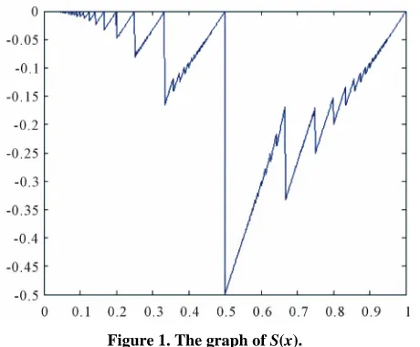
Figure 1. The graph of S(x).

4. Acknowledgements

This work is s ion De

[1] S. Kalpazidou, A. Knopfmacher and J. Knopfmacher, “Lü roth-Type Alt entations for Real Numbers,” Ac , No. 4, 1990, pp.

No. 3, 1991, pp. 319-325.

p. 311-

ol. 8, No. 2, 1996, pp. 331-346. B44, 1992, pp. 17-28.

[3] S. Kalpazidou, A. Knopfmacher and J. Knopfmacher, “Me- tric Properties of Alternating Lüroth Series,” Potugaliae Mathematica, Vol. 48,

[4] J. Barrionuevo, M. Burton-Robert, Dajani-Karma and C. Kraaikamp, “Ergodic Properties of Generalized Lüroth Series,” Acta Arithmetica, Vol. 74, No. 4, 1996, p

327.

[5] K. Dajani and C. Kraaikamp, “On Approximation by Lü- roth Series,” Journal de Théorie des Nombres de Borde- aux, V

doi:10.5802/jtnb.172

[6] K. J. Falconer, “Fractal Geometry, Mathematical Founda- tions and Applications,” Wiley, Hoboken, 1990.

06, pp. 223-232. [7] K. J. Falconer, “Techniques in Fractal Geometry,” Wiley,

Hoboken, 1997.

[8] J. Galambos, “Reprentations of Real Numbers by Infinite Series,” Lecture Notes in Math, Springer, Berlin, 1976. [9] L. M. Shen and J. Wu, “On the Error-Sum Function of

Lüroth Series,” Mathematics Analysis and Applications,

Vol. 329, No. 2, 2007, pp. 1440-1445.

upported by the Hunan Educat part-

ment Fund (11C671).

[10] L. M. Shen, C. Ma and J. H. Zhang, “On the Error-Sum Function of Alternating Lüroth Series,” Analysis in The- ory and Applications, Vol. 22, No. 3, 20

REFERENCES

doi:10.1007/s10496-006-0223-x

[11] T. Sálat and S. Znám, “On the Sums of Prime Powers,”

Acta Universitatis Palackianae Olomucensisof Mathema-tica, Vol. 21, 1968, pp. 21-25.

- ernating Series Repres

ta Arithmetica, Vol. 55

311-322.

doi:10.5802/jtnb

doi:10.1007/s10496-006-0223-x