warwick.ac.uk/lib-publications
A Thesis Submitted for the Degree of PhD at the University of Warwick
Permanent WRAP URL:
http://wrap.warwick.ac.uk/106494/
Copyright and reuse:
This thesis is made available online and is protected by original copyright.
Please scroll down to view the document itself.
Please refer to the repository record for this item for information to help you to cite it.
Our policy information is available from the repository home page.
RATIONAL EXPECTATION MODELS
by
Paul Gregory Fisher
Thesis subm itted for the degree of Doctor of Philosophy
to the
UNIVERSITY OF WARWICK Department of Economics
CONTENTS
Page
Contents i
List of tables and figures iv
Acknowledgements vi
Declaration vii
Summary viii
Abbreviations ix
1. INTRODUCTION 1
1.1 Objectives of the thesis 2
1.2 Outline of the research 4
2. LARGE SCALE MACROECONOMIC MODELS AND 6
FORWARD EXPECTATIONS 6
2.1 Large—scale models of the economy 10
2.2 Solution and simulation of macroeconomic models 13
2.3 Stochastic simulation 16
2.4 Optimal control 20
2.5 The role of expectations 21
2.6 The solution of forward expectations models 26
2.7 Uniqueness, stability and terminal conditions 31
2.8 Time inconsistency 33
2.0 Control and policy analysis 40
Page
3. SOLUTION METHODS FOR NONLINEAR FORWARD 42
EXPECTATIONS MODELS
3.1 First order iterative solution techniques 43
3.2 Nonlinear models 45
3.3 Forward expectations models 46
3.4 The iterative schemes 50
3.5 Empirical results 55
3.6 Penalty function methods (Newton’s method) 60
3.7 Comparative costs of the penalty function method 64
3.8 Shooting techniques 67
3.9 The feasibility of shooting techniques 74
3.10 Comparative analysis of the shooting method 77
3.11 S u m m ary 83
4. TERMINAL CONDITIONS, UNIQUENESS AND STABILITY 84
4.1 Uniqueness and stability conditions 84
4.2 Terminal conditions in the Unear model 90
4.3 The impUcations of terminal conditions for model solution 101
4.4 Empirical results: AppUcations to large-scale models 105
4.5 Conclusions 126
5. EXPERIMENTAL DESIGN AND STOCHASTIC SIMULATION 128
5.1 Anticipated and unanticipated shocks 129
5.2 Anticipated and unanticipated shocks: empirical results 133
5.3 Temporary and permanent shocks (poUcy reversal) 139
5.4 Temporary and permanent shocks: empirical results 141
5.5 Stochastic simulation 145
5.6 Empirical results: stochastic simulation 152
i l i
Pige
6. ALTERNATIVE MODEL FORMS AND SOLUTION MODES: 162
HISTORICAL TRACKING
6.1 Conventional models 162
6.2 Forward expectation models 167
6.3 Historical tracking 171
6.4 Static and dynamic simulation residuals 174
6.5 The historical tracking record of the models 178
6.6 Cross—model comparisons 198
6.7 Using the models for counter-factual simulations 205
6.8 Summary and conclusions 207
7. CONTROL AND POLICY ANALYSIS: EXPERIMENTAL DESIGN 210
7.1 Optimal control algorithms for forward expectations models 210
7.2 Calculating trade-offs 222
7.3 In flatio n —unem ploym ent tra d e -o ffs: em pirical resu lts 233
7.4 Summary and conclusions 243
8. CONCLUSIONS 244
8.1 Summary 244
8.2 Directions for future research 246
». BIBLIOGRAPHY 248
LIST OF TABLES AND FIGURES
Tables Page
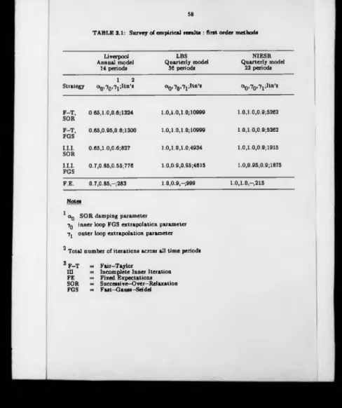
3.1 Summary of empirical results for iterative solution methods 58
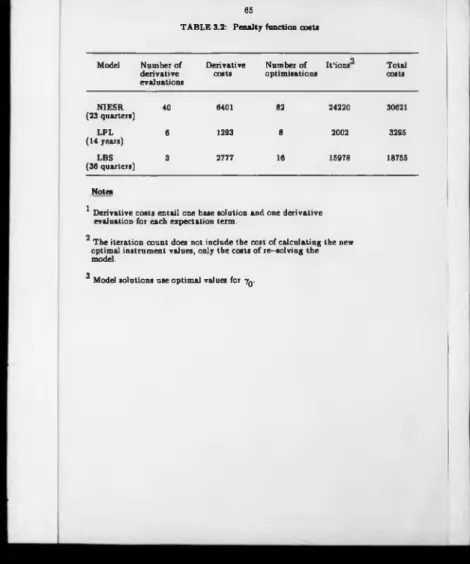
3.2 Penalty function costs 65
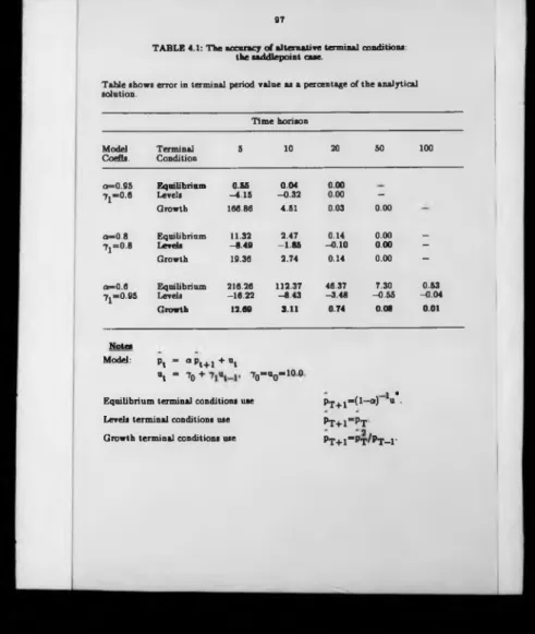
4.1 The accuracy of alterative terminal conditions: the saddlepoint case 97
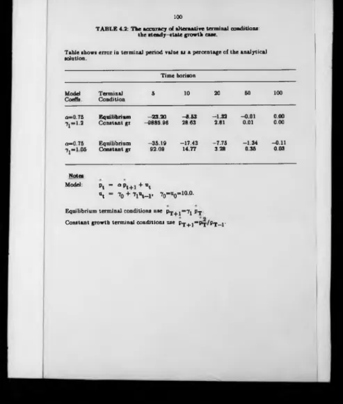
4.2 The accuracy of alternative terminal conditions: 100
the stea d y -state growth case
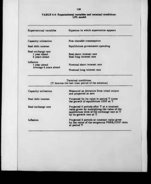
4.3 Summary of convergence results for alternative terminal values 106 4.4 LPL model: expectational variables and term inal conditions 108 4.5 LBS model: expectational variables and terminal conditions 116 4.6 NIESR model: expectational variables and term inal conditions 119
5.1 Stochastic simulation of the NIESR model 155
5.2 Stochastic simulation of the LBS model 157
5.3 Stochastic simulation of the LPL model 159
6.1 Static simulation residuals, summary statistics 180
6.2 Theil inequality coefficients 200
6.3 Forecasting encompassing tests, annual models 203
6.4 Forecasting encompassing tests, quarterly models 204
7.1 Specification of the objective function 234
Figures Psge
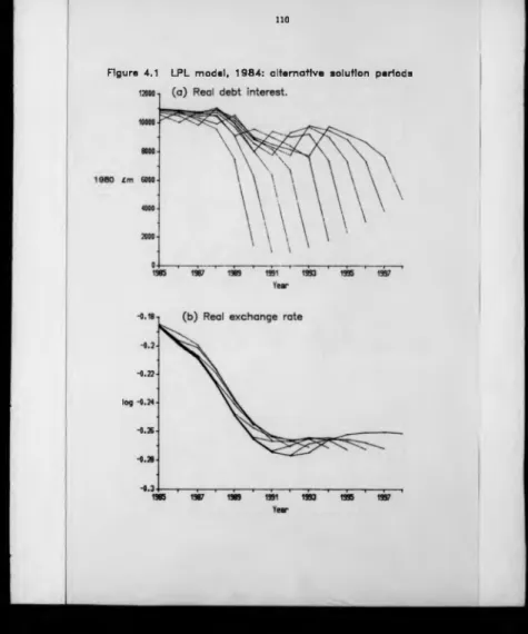
4.1 LPL model: alternative solution periods 110
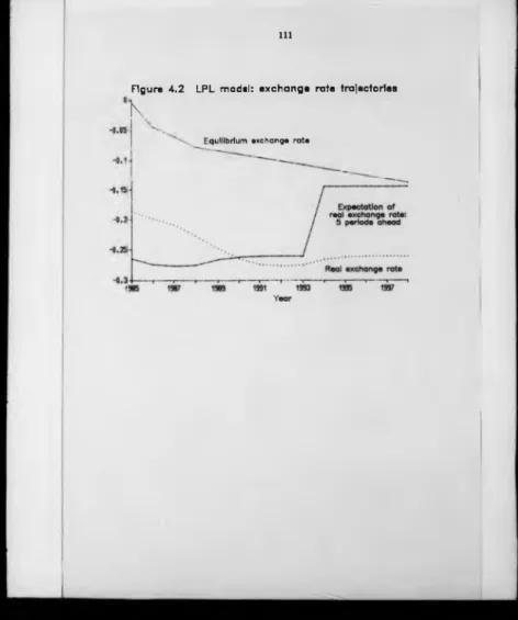
4.2 LPL model: exchange rate trajectories 111
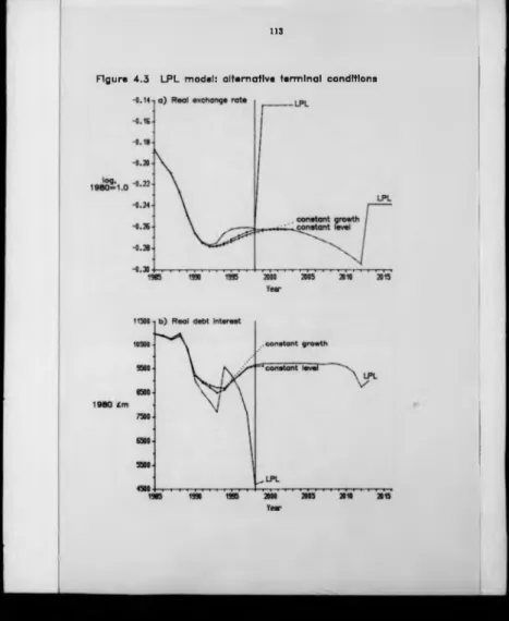
4.3 LPL model: alternative terminal conditions 113
a) Real exchange rate b) Real debt interest
▼
P**e
4.5 LBS model: price of gilts 117
a) Alternative solution periods b) Alternative terminal conditions
4.6 NIESR model: alternative solution periods: 121
effective exchange rate
5.1 Comparison of anticipated and unanticipated shocks: NIESR model 135 5.2 Comparison of anticipated and unanticipated shocks: LBS model 136 5.3 Comparison of anticipated and unanticipated shocks: LPL model 138 5.4 Comparison of temporary and permanent shocks: NIESR model 143 5.5 Comparison of temporary and permanent shocks: LBS model 144 5.6 Comparison of temporary and permanent shocks: LPL model 146
6.1 The historical data record 1978-1985 179
6.2 BE model: static simulation residuals 182
6.3 HMT model: static simulation residuals 184
6.4 NIESR model: static simulation residuals 187
6.5 NIESR model: variant assumptions 188
6.6 LBS model: static simulation residuals 190
6.7 LBS model: variant assumptions 191
6.8 LPL model: static simulation residuals 193
6.9 LPL model: variant assumptions 194
6.10 CUBS model: static simulation residuals 197
7.1 Trade-off calculations 226
7.2 LBS model: optimised inflation—unemployment trade-off 236
7.3 NIESR model: optimised inflation—unemployment trade-off 238
This thesis has been developed during the course of the research programme of th e ESRC Macroeconomic Modelling Bureau, partially in response to the needs of th a t work. Indirect support by the ESRC is therefore acknowledged. Special thanks are due to my supervisor and the director of the Bureau, Professor K .F. Wallis and to the Bureau's principal research fellow Dr. J.D. Whitley. I am also grateful for the comments and encouragement of Bureau colleagues M .J. Andrews, D.N.F. Bell, A.J. Longbottom, S.K. Tanna, and D.S. Turner. Thanks are also due to co-authors on particular topics: Professors A. J. Hughes Hallett and M.H. Salmon.
VII
DECLARATION
Some of the results presented in this thesis have already been published in jointly authored work. Specific acknowledgements are due as follows. Chapter 3, sections 3.1, 3.2 and 3.4 and the LPL and LBS results of section 3.5 are revised material from Fisher and Hughes Hallett (1988). Professor Hughes Hallett was primarily responsible for developing the analysis in sections 3.1, 3.2 and 3.4. These sections are the only material in the thesis not primarily the work of the author and are included for completeness. The author was responsible for the proposal and implementation of the general approach to incomplete inner iteration strategies including the precise technique employed and the generation of the results in section 3.5. The NIESR results in 3.5 and all of sections 3.6, 3.7, 3.8, 3.9 and 3.10 are new work.
This thesis presents a comprehensive set of techniques for solving, simulating, analysing and controlling large scale, nonlinear, econometric models th a t contain rational expectations of future dated variables. These expectations are generally treated as model consistent, whereby the expectation is set to the deterministic projection of the model.
Solutions to such models are distinguished from those of conventional models by the fact that they are not recursive in time. The outcome for the current period depends on the expected outcome for future periods as well as past periods. This property means that all of the basic numerical procedures need to be altered.
We consider the following topics: solution algorithms for the two—point boundary value problem; terminal conditions, uniqueness and stability; experimental design and stochastic simulation; model forms, solution modes and historical tracking; control methods including optimal control. We find that suitable procedures allow us to undertake all of the experiments usually conducted with conventional models.
ix
ABBREVIATIONS
BE Bank of England
CUBS City University Business School
EEC European Economic Community
FGS Fast Gauss—Seidel
FIML Full information maximum likelihood FOI First order iterations
FT Fair—Taylor
FWW Fisher, Wallis and Whitley
GDP Gross domestic product
HMT Her Majesty’s Treasury
III Incomplete inner iterations
IV Instrumental variables
JOR Jacobi—over—relaxation
LBS London Business School
LPL Liverpool Research Group in Macroeconomics
MAE Mean absolute error
NIESR National Institute of Economic and Social Research NPV Net present value
OLS Ordinary least squares
PSBR Public sector borrowing requirement RMSE Root—mean-square error SOR Successive-over-relaxation
UK United Kingdom
US United States of America VAT Value added tax
INTRODUCTION
Throughout the last two decades, expectations formation has been a t the heart of macroeconomic research. In particular, following the work of Muth (1961), attention has been concentrated on the concept of rational expectations i.e. th a t agents form expectations consistent with their knowledge of the underlying processes of the economic system and taking into account all available information. The rational expectations hypothesis has sufficiently penetrated all areas of macroeconomic theory and applied work to have caused a "revolution in macroeconomics" according to Begg (1982). Developments in macroeconomic theory are usually incorporated, sooner or later, into large-scale macroeconomic models. In the United Kingdom there are now three large, nonlinear, empirical, macroeconomic forecasting models which incorporate rational expectation terms as part of their basic structure.
The Liverpool model (LPL) is an annual model which has been based on rational expectations since its inception in 1979. It is new classical in structure with a set of long-run equilibrium equations determined only by the supply side. The London Business School (LBS) and National Institute of Economic and Social Research (NIESR) models are quarterly and used rational expectation models for their forecasts for the first time during 1985 (Economic Outlook, October; National
Institute Economic Review, November). The LBS model has three expectation
2
The actual processes by which agents form expectations are generally unknown and their precise expectations concerning future macroeconomic quantities are usually unobserved. The assumption of rational expectations in economic theory therefore leads to complications both in estimating equations which contain explicit expectation terms and in the numerical procedures which are designed to solve, simulate and analyse large-scale models which contain such terms. The econometric literature now suggests a range of statistical methods which allow the estimation of equations containing rational expectation terms (e.g. see Begg, 1982, Ch.5). This thesis concerns numerical methods which allow the use of such equations in large-scale models.
1.1 The objectives of the thesis
The primary objective of this thesis is to establish a set of numerical methods for the simulation, analysis and optimal control of large-scale, nonlinear, macroeconomic models that contain rational expectations of future-dated variables. These methods allow us to undertake on rational expectations models all of the experiments usually performed with conventional large-scale models such as forecasting, policy analysis or stochastic simulation.
Numerical methods are often designed for specific problems or for specific models. In this thesis we aim to establish a general set of techniques which can be applied to a variety of models and problems. Starting from these general methods we can then modify the procedures to suit the requirements of particular experiments.
The secondary objective of the thesis is to use our procedures to investigate the properties of the three publicly available models of the U K. economy which incorporate rational expectations terms. As noted by Wallis (1987):
those models with rational expectations may not coincide with the new-classical model. The elucidation of the properties of these models is therefore of some interest.
In the three different U.K. models containing rational expectations, the only common expectations term is that of the sterling effective exchange rate. In a relatively small open economy, operating under a floating rate regime, fluctuations in the exchange ra te can be a particularly im portant transmission mechanism. Expectations of future exchange rates changes appear to play an important behavioural role in determining its current value (Isard, 1988) and these terms are therefore of fundamental importance to the properties of U.K. models (e.g. see Wallis et al., 1987, pp44-48). When explaining our results we pay particular attention to the behaviour of the exchange rate.
In Chapter 2 we present a wide-ranging literature survey covering all aspects of large-scale modelling but paying particular attention to the numerical methods used. The role of expectations is discussed and we consider the problems caused by including expectation terms of future-dated variables. We conclude that the issues raised have only partially been resolved by the existing literature. Some problems, such as terminal condition choice, do not appear to have been considered in depth and some existing numerical methods, such as those for the optimal control of nonlinear rational expectations models, do not appear to be well understood.
4
alternative approaches to solving nonlinear rational expectations models. In Chapter 4 we address the issues of uniqueness and stability in the solutions of rational expectations models. Having established th e conditions for a unique stable solution to exist, we are faced w ith the problem of locating that solution. This comes down to the choice of term inal values for the expectation terms in the final solution period. A number of possible terminal conditions are proposed and evaluated on both a small demonstration model and the three la rg e- scale models. Particular attention is paid to th e implications of different choices when there is not a unique stable solution.
The following chapter begins by examining the implications of different assumptions concerning input shocks. Such shocks may be introduced for the purpose of policy analysis or simply to evaluate th e partial responses of the model. The shock can be treated as anticipated or unanticipated, temporary or permanent. The practical implications of such distinctions are evaluated for each of the three large-scale models.
The analysis of a sequence of temporary, unanticipated shocks leads us to a proposed method of stochastic simulation which differs from two methods proposed elsewhere in the literature. The differences are critically assessed and our preferred method is applied in an experiment to reveal the stochastic implications of alternative assumptions for the financing of the PSBR.
In Chapter 6 we present a general discussion of alternative model forms (structural form, reduced form, final form) and solution modes (single-equation, static, dynamic) extended to the rational expectations case. In particular we develop an appropriate method for the static simulation of rational expectations models. We argue that static rather than dynamic simulation is the correct procedure to be used in evaluating the historical tracking performance of models. A comprehensive historical tracking exercise is presented for six U.K. models, three containing rational expectations and three without.
produce the optim al solutions corresponding to different formulations o f the policy optimization problem. The differences in these solutions are discussed an d critically assessed. One of the three algorithms is then used to derive optim al inflation- unemployment trade-offs for the three large-scale rational expectations models. Attention is paid both to the observed economic properties of the models and the costs of the optimization procedure. Finally, the implications are examined of alternative formulations of the problem.
Chapter 2
LARGE-SCALE MACROECONOMIC MODELS AND FORWARD EXPECTATIONS
In this chapter we begin by reviewing the nature and purpose of large-scale macroeconomic models. We then survey the development of the rational expectations literature and lead in to large-scale macroeconomic models with forward expectations. We consider the problems posed for conventional numerical methods in solving, simulating and analysing these models and the extent to which these problems are overcome by existing procedures.
2.1 Large-scale mods»» of the e w no ai
a set of macroeconomic aggregates such as consumption expenditure, th e general price level or the exchange rate between domestic and foreign currency. We condition our model by choosing not to explain certain other aggregates on economic or statistical grounds. We may exclude certain policy variables (e.g. th e rate of interest in some models); those which are determined outside the geographical economy of interest (e.g. world production if we are modelling the U.K.); or simply those variables which are within the system but which are not of interest to the user of the model (e.g. some demographic factors such as the birth rate).
The relationships between the variables being explained by th e model (the endogenous variables) and those not being explained (the exogenous variables) are modelled using algebraic representations. These models then consist of a system of simultaneous equations. These equations may be derived entirely from theoretical analysis or they may have functional forms and/or numerical parameters which are based on empirical exercises. Models based on empirical research, often distinguished by the term "macroeconometric models" will usually be based on time series d ata recorded over some historical period. This gives the model builder a choice of temporal aggregation, usually annual or quarterly although continuous time models have also been developed (e.g. Bergstrom, 1967; Gandolfo, 1981).
The first macroeconomic model was presented by Jan Tinbergen over fifty years ago (Tinbergen 1936). In the period since, there have been many models developed for a range of purposes. In particular we identify three main uses of a large-scale macroeconomic model: understanding the processes of the economy; predicting the future course of the economy (forecasting); analysing the effects on the economy of external shocks or changes in policy variables. For th e U.K. some recent developments in these areas have been surveyed by Wallis (1988, 1989).
8
individual model may still depend on the way in which it is used: the answer depends on how the question is asked. This aspect is discussed by Turner, Wallis and Whitley (1989). A classic example is th a t the effects of an increase in government expenditure depend on how it is financed: by printing money, issuing debt or raising taxes. This particular example has its roots in the seminal papers of Christ (1968) and Blinder and Solow (1973).
Macroeconomic models are built to give a detailed representation of the economy and may range from just one or two equations up to many thousands (the project LINK model of the world economy contains some 20000 equations: Petersen, 1987). The definition of what size model comprises large-scale is somewhat arbitrary. The smallest model used in this thesis contains just 30 equations and the largest just over 1200. Large models are often multi-purpose, designed for all three of the activities noted above. The costs associated with building and maintaining a model increase with size and there is an obvious incentive to extract the maximum use value.
Each equation in a large model will be grounded to a greater or lesser extent in an economic analysis of a particular behavioural relationship. Typically the majority of equations in the model will be estimated. T hat is to say, they have functional forms, numerical coefficients and a choice of explanatory variables which are determined to some extent by the use of econometric methods. In this thesis we shall be largely treating the structure of models as given. The process of constructing models is covered in texts such as Fair (1984) and Holden, Peel and Thompson (1982).
The simplest representation of an economic system is a set of linear, static equations which we may write as:
B ^ + C x j - U j , (2.1)
vector of disturbance terms. The matrices B and C are (n«n) and (n*m) matrices of coefficient values respectively (derived or estimated). The n elements of ut (ujt , i= l,...,n ) are non-zero whenever equation i does not perfectly fit the observed data in period t. An equation j for which Ujt = 0 in every period t= l,...,T is defined as an identity. A system for which B is diagonal is un-coupled or non-simultaneous. Off-diagonal elements in B represent the direct effect of the outcome of one decision on another.
In general, economic behaviour is dynamic in the sense that decisions made in period t depend on past decisions and conditioning information to rn earlier periods as well as xt . A general dynamic model can be represented by use of the lag operator L which is defined such th at Lyt = yt_ j- We can then generalize equation (2.1) to:
where B(L), C(L) are now matrices of polynomials of order p, q repectively such th»l B(L) r t - BQyt + B j j ^ j + B2jrt_ j + ... + B ^ j , ^ and C(L) i> Bmilarly
Equation (2.2) still presents the model in linear form whereas in practice, most large-scale models involve nonlinear relationships. Examples include log—linear equations in which the variables are first transformed by taking logs or ratio transformations such as taking the current account balance as a fraction of total output in forming an explanatory variable. A combination of linear identities, log-linear equations and multi—variable transformations together with the occasional extreme nonlinearity (such as raising to a power) will typically yield a system which cannot be expressed in the form of equation (2.2). We therefore adopt a more general notation:
B(L) y , + C(L) x, = u , (2.2)
defined.
10
The vector of general functions f( •) is restricted only in th a t it is a real—valued function of real variables. The vectors defined with capital letters and Yt _ j represent all observations up to the date indicated i.e. X ' = { x ', x ' _ j , ... , x '_ ^} and Y '_ j = { y '_ j, y ' _ .. . , y^_p} . The vector 6 represents all the parameters of f(•) and 0^ will represent the parameters of equation f (• ) . Although the vast majority of large-scale models are nonlinear, the linear forms (2.1) and (2.2) can still be useful as an analytical device for considering the behaviour of the nonlinear system (2.3). The linear system (2.2) could be considered as a first order approximation to th e nonlinear system (2.3) in some local neighbourhood of its solution. The elements of B(L) and C(L) are then interpreted as partial derivatives of f(-). Hence in some parts of the exposition we continue to use the linear form (2.2) and this has the benefit th at linear systems are easily manipulated to give closed form expressions whereas general nonlinear systems are not.
The use of a model for understanding the processes of th e economy is partly a matter of examining the specific relationships embodied in th e system. However, there are also various experiments which we may wish to conduct such as full system analysis, policy analysis or forecasting and these exercises require a set of numerical techniques for solving and simulating the model. The computational complexity of these techniques generally increases as we move from models of the form (2.1) through (2.2) to (2.3). Throughout this thesis, a detailed presentation of techniques will be made as we extend them to cover the forward expectations case. In this section we briefly summarize these procedures for models of the form so far considered.
essential requirement. Solution procedures are covered by many authors e.g. Hughes Hallett and Rees (1983).
The static linear system (2.1) can be used to solve for y( , t= l,...,T for each t by obtaining th e reduced form solution:
7t - - B - 1 C X , + B- 1 u ,. (2.4a)
Hence the only numerical technique needed is th e inversion of B which is required to be of full rank. In what follows, we assume th a t the disturbances (u( ) are set to zero for simplicity. For the dynamic model (2.2) we can solve for a static or dynamic sequence. In the static sequence the lagged values yt_ j,. -,yt_ p are set to observed historical values and the system is solved for y^. In the dynamic sequence, the solution value for y^ is calculated using observed historical values but the solution for y j then depends on the solved value for y^. The solution for yt , t> p uses solution values for all the lags on y. These solutions can be expressed as:
U ~ ~ * 0 I V t - l + + V t - p + C0*t + ••• + V t —q] (J -4b)
y, - -B o1 I V t - I + - + Bpyt- p + c o*t + - + c ,* t_q l (2 4c) t = l ...T
yt - s “
for the static and dynamic solutions respectively. For dynamic as well as static systems the reduced form solution is obtained by matrix inversion. For large systems this inversion can be costly and the solution is usually obtained by solving the simultaneous equation system by direct methods which will be discussed below. In both cases we require BQ to have full rank. The dynamic system need not be stable but the stability condition requires that the determinantal polynomial | B(L) | has all its roots of modulus less than unity.
12
convenient expression. Instead we assume that th e conditions of the implicit function theorem hold and we write the reduced form of equation (2.3) as:
y , = s ( V r x t ■ ut' «) (2-o>
In general there may be more than one solution to equation (2.3) which satisfies equation (2.5) but of all the large-scale models there has been only one case of multiple solutions arising from nonlinearities reported in the literature (Friedman, 1971). Since the function g(-) is not usually obtainable analytically, we solve equation (2.3) directly by numerical methods. For some of the methods considered below we require th a t we can re-w rite equation (2.3) as:
y , = M y,; x (i *). (2.6)
As in the linear case, we set ut = 0 for simplicity. In the nonlinear case however, this causes complications which we consider in the next section.
Solutions to the system (2.3) or (2.0) are typically generated either by derivative—based methods or first-order iterative methods. The commonest derivative—based technique is the Newton method. To obtain this numerical algorithm we consider an expansion of the i’th equation in system (2.3) around some trial solution y ^ :
y ) - j £ i [« i/«yj] | y(0).(yr yj(0)) - o. (2.7)
Solving equation (2.7) for i= l,...,n simultaneously yields the iteration:
First-order methods are based on solving equation (2.6). These methods will be considered in greater depth in Chapter 3 but the simplest form, the Jacobi method, can be obtained by simply writing equation (2.6) as:
j j 0 - ‘■(Jt (,_1); X,; u( ; t) (2.8)
For both derivative-based and first-order methods, the solution yt is found when
where r is some chosen tolerance level.
In the two algorithms given above, the ordering of the equations i= l,...,n is irrelevant. Gabay et aL (1980) and Don and Gallo (1987) have shown that the efficiency of th e Newton solution procedure can be improved by exploiting any sparseness (zero entries) of the F matrix to reduce the dimensionality of the matrix inversion in equation (2.8). Hughes Hallett and Fisher (1987) have shown that any such observed sparseness can be used to re-order the equations to improve the efficiency of general first-order methods.
The solution methods discussed in this section are the basic tool used in the simulation of macroeconomic models. They allow us to calculate th e values of the endogenous variables yt conditional on alternative values for the exogenous variables x^ — which might be actual or forecast values; an hypothesized policy setting or simply a shock to the system . In addition we will consider two further types of simulation which require more complicated techniques: stochastic simulation and optimal control.
2.3 SiochMtic Bmalatiop
14
period is a property of most econometric estimators. If an equation is observed to have residuals with a non-zero mean (e.g. post-sample) then an estimate of the mean value is sometimes used rather than zero. In either case, these solutions are defined as deterministic because they offer a single point estimate of yt ignoring the stochastic nature of the system. A stochastic simulation is an (Monte Carlo) experiment undertaken with a model in order to approximate the distribution of y( .
It has been known, at least since Howrey and Kelejian (1971), that the deterministic solution to a nonlinear model is generally a biased estimate of its conditional expectation. This arises because the expectation of a nonlinear function of a random variable is not generally equal to the same function of the expectation of th a t variable i.e.
E( g(Yt_ i; X,; u,; 0)) * g(Yt_ , ; X( ; Efu,); 0). (2.10)
Furthermore, the deterministic solution to equation (2.3) gives us no information on the distribution of yt unlike the linear model (2.1) in which, for example, the conditional variance-covariance m atrix of yt can be obtained directly as Bq**^Bq* (where 4»t = E(ut Uj)) and hence estimated from the residuals ut = y t~yt (where yt denotes the fitted value of the estimated equation). Stochastic simulation can be used to obtain an unbiased estim ate of the conditional expectation of g(-) and estimates of the higher order moments.
vector of pseudo—random standard normal deviates T . .
and for an estimated variance—covariance matrix ♦ = £ u .u r /T we obtain a set of disturbances
. t=1
s(r>' = v j^ 'W where W 'W = ♦ . This method is unfortunately not generally feasible because the required decomposition of the covariance matrix is only obtainable when th a t matrix ( ♦ ) is non-singular. We seldom have enough degrees of freedom to identify all the (n * (n + l))/2 parameters involved in the covariance matrix.
The McCarthy method (McCarthy, 1972) is the most commonly adopted residual generation technique for stochastic simulation of large systems. It overcomes the problem of the Nagar procedure by using th e residuals directly instead of decomposing the variance-covariance m atrix to generate the pseudo-random shocks i.e. s |r ) = T- v ^ U where U is th e (T«n) matrix of observed residuals and vjr) is now a (T *l) vector of pseudo—random standard normal deviates. This procedure generates disturbances w ith a covariance matrix which, for large R, tends to that of the residuals. This procedure can be extended to include the serial correlation properties of u^; details are given in Schink (1971). For estimating th e bias of the deterministic solution we calculate the difference between that value and the mean of the stochastic replications (which is our estimate of the conditional expectation). This estimates the ex ten t of the inequality in equation (2.10). Calzolari (1979) has suggested a method of negative antithetic variates which helps to reduce the experimental variance in estimating the bias. Calzolari and Sterbenz (1989) have recently proposed a generalization of the McCarthy procedure which explicitly maintains the empirical third moment of the disribution of the residuals.
16
resulting distribution of the shocks is therefore identical to the historical distribution. By sampling randomly and repeatedly from the observed residuals, this procedure becomes a boot-strap type method (Mariano, 1985).
Fisher and Salmon (1986) present a survey of stochastic simulation experiments and examine the implications of changes in the experimental design for the measurement of the bias. This survey is reproduced and slightly extended in Hall and Henry (1987). Fisher, Wallis and Whitley (1985) use stochastic simulation to estimate second moments and their results are extended in this thesis.
2.4 Optimal control
Control theory is a subject area that covers a wide spectrum of techniques which, in the economics literature, is aimed primarily at policy optimization (e.g. Chow, 1975, 1981). In the context of large-scale, nonlinear macroeconomic models, optimal control is a term usually used to indicate a particular numerical technique for the analysis of policy which is optimal in some explicit sense. However, optimal control can also be viewed as a method of generating simulations or as an aid to full system analysis.
trajectory, ceteris paribus, for xt , t« l,...,T .
For linear models there is a substantial literature covering methods for the optimal and sub-optim al control of economic systems. These techniques were originally developed in the engineering literature and adapted for economic systems because of their mathematical similarity to physical systems (see e.g. Chow 1975, 1981; Holly, Rustem and Zarrop (eds.) 1979). We therefore begin by summarizing the basic results of this literature.
We begin by re-writing the general dynamic model (2.2) as:
y, = B y ,_ j + C x , + D 2, + u , (2.11)
where we have separated out a vector of policy variables zt from the other exogenous variables (x^). The dynamics in (2.2) are reduced to first-order terms only by defining new variables dated t for the longer lags. The y and x vectors in equation (2.11) are then no longer the same as those in equation (2.2). There is no unique way of reducing a general dynamic model to a first-order system but various state-space forms are popular (e.g. see Aolri, 1976).
In formulating a control problem, we set up a formal explicit objective function which specifies the desired trajectories for both endogenous variables (henceforth targets) and exogenous variables (henceforth instruments) as well as the costs associated with deviating from the desired paths. The most common approach is to use a quadratic function such as:
Jt = * J t i( y t - y t) 'w y t(y ry t) +( * t - i t ) ' w x ( 212>
18
since equation (2.11) has a stochastic disturbnance term. However, we ignore the stochastic component in what follows. The optimal values can be determined in the form of a linear control rule:
*t = Kt yt - l + *Y (213)
where K^, known as the feedback gain, and h( known as th e tracking gain (or feedforward term ) can be expressed in closed form as functions of the model parameters, the weighting matrices and the desired values (for all time periods) see e.g. Holly and Hughes Hallett (1989, pp41—42). The feedback rule is complicated and time—varying. The precise form of these expressions is therefore only of relevance in obtaining the optimal values.
In 1978 the Committee on Policy Optimization chaired by Professor R. J. Ball reported to Parliament on the possible application of optimal control techniques to Her Majesty’s Treasury’ macroeconomic model (Cmnd. 7148, 1978). For such nonlinear models there are no closed form analytical solutions available. In the following presentation we therefore resort to a linear model from which we can derive nonlinear methods.
We now write the economic model in stacked form as:
D Y + E X = U, (2.14)
where D and E are the parameter matrices containing the system matrices (2.2) stacked over tim e and (Y, X) denote vectors of observations stacked over time such that: Y ' = {y£, y£, ... ,y£) and y( and x( are now the same vectors as in equation (2.2). We also stack the objective function over time:
J = * (Y -Y )'W y(Y -Y ) 4- * (X -X )'W x(X -X ) . (2.15)
are (nT «nT ) and (mT*mT) repectively and are chosen to be positive semi-definite and elements of y or x th a t are not targets or instrum ents have zero weights attached. The objective function J is then minimized subject to the constraint imposed by the model (2.14). The optimal solution can be found by substituting the constraint (2.15) into th e model (2.14) and differentiating the resulting function directly to obtain optimal values (Y°, X°) from the first order conditions and hence:
x ° = [ n - w y n + w j -1 [w xx + n - W y Y - n 'W y D ^ u ] (2.16a)
Y ° = -D _ 1 ( E X ° - 0 ) (2.16b)
where II = —D— . For a nonlinear system, we obtain the minimum of the objective function J by numerical means as follows. Taking the function (2.15) and substituting in the model (2.14) we have a general nonlinear function. This can be minimized using derivative—based methods as for the basic solution problem in solving th e nonlinear model (2.3). In practice the dimension of this resulting equation system is so huge (even for just a few instrum ents/targets) th a t more efficient approximations to Newton’s method are used. Rustem and Zarrop (1979, 1981) propose various quasi—Newton algorithms for minimizing J subject to a general nonlinear model.
In general the equations given by (2.16) are simply another way of writing the feedback control rule. However, in the numerical approach there is no attempt to form ulate the solution as a linear control rule - the result is simply a set of optim al values for x( and hence y( . The other distinguishing feature is th a t (2.16) solves for all time periods simultaneously whereas (2.13) can solve for a single period (as a function of desired values and weights in all periods).
20
use optimal control analysis to derive output—inflation trade-offs in the manner of Chow and Megdal (1978). This form of analysis is to be examined and extended in Chapter 7.
2.5 The role of expectations
The role of expectations in macroeconomic relationships has long been recognized. In Keynes’ General Theory (1936) th e influence of expectations received much explicit attention. There is one chapter considering "Expectation as determining output and employment." and another on "The state of long-term expectation." . In his "General theory of the rate of interest.", Keynes offered a detailed example which is now used as a standard introductory explanation of investment behaviour. An investment project will be profitable if its discounted stream of net revenues is positive. This Net Present Value may be defined in terms of revenues R, costs C and discount factor d over the life of a project (T years) by the formula:
NPV ■ , l o (Rt“ C«)/( 1 + d t ) (J1T)
However, in an uncertain world the values of Rt , Ct and dt are not known in the initial period 0. Hence the NPV is evaluated using expectations of these variables. Therefore investment decisions m ust depend on expectations of the future.
The treatment of expectations in the economics literature initially developed slowly. An important early contribution was made by Grunberg and Modigliani (1954) who showed how forecasts could be self-fulfilling if one takes into account the reactions of agents to th e forecasts. The modern literature on "rational" expectations is often assumed to start with Muth (1961). It was M uth who coined the phrase and declared a rational expectation to be (p46):
In the context of a system of algebraic equations subject to a random disturbance term, this is interpreted in mathematical terms as the appropriate conditional expectation.
The rational expectation of a variable yt formed in period s<t and based on a particular theory or model is distinguished from other mechanisms for generating expectations such as extrapolative forecasts. Adaptive expectations are a particular land of extrapolative forecast which are also considered by M uth. The adaptive expectation denoted y* may be expressed in the following manner:
y? = y ,_ , + A(yJ_, - yt_ j) (2.18)
for some parameter 1>A>0. Hence the adaptive expectation o f yt is a function of its own past and is essentially an adjustment mechanism designed to use information on past errors to improve current forecasts.
The rational expectation of variable yt formed in period s<t will be denoted yt | g and defined as E(yt | n g): the conditional expectation of yt given the information set fig. The information set is assumed to contain all data on the variables of the model which are available at the end of period s and the relevant model (or theory). The information set could alternatively be defined for the beginning of a period and dated appropriately for the context. In Muth’s simple example the adaptive expectation and the rational expectation coincide but this is a very special case.
22
th a t no such relationship exists. The long-run trade-off between output and inflation in Lucas and Rapping’s model becomes non-existent as inflation expectations match actual inflationary changes. This model then helped to explain the observed breakdown in the output-inflation relationship which occurred in th e 1960’s. Lucas and Rapping explicitly reject the assumption of rational expectations but the primary importance attached to the role of expectations opened the way for later developments.
During th e 1970’s, the rational expectations hypothesis was adopted as an integral part of the new-classical economics. Particularly important contributions were made, inter alia, by Lucas (1972 a,b; 1973; 1975), Sargent (1973, 1976), Sargent and Wallace (1973, 1975, 1976), Barro (1976, 1977) and Kydland and Prescott (1977). These authors combined rational expectations with new—classical macroeconomics and the policy ineffectiveness proposition. An excellent survey and critique of this literature is given by Shiller (1978). Following the theoretical literature, rational expectations began to appear in small macroeconomic models (e.g. Sargent, 1976; Taylor, 1979).
As the explicit treatm ent of expectations became more common, an im portant distinction was made between different types of expectations variables. In particular we shall now consider forward expectations (e.g. yt+ 1 | t_ j) and current expectations e.g. (yt |t_ i) - Let us consider a wage equation in which nominal wages (W() depend on expectations of prices in the current period formed in the previous period so that we have Wt =w(pt | t_ j) . We call this a current expectations term. As mentioned above, we may alternatively consider the current expectation to have been formed using information available at the start of period t and hence write Wt =w(pt | t ). This difference is simply a question of dating the information set according to the underlying economic theory. However, as discussed by Aoki and Canzoneri (1979), the forward expectation is different in kind. In this case we assume th at wages are a function of the expectation of next period’s prices: Wt = w(pt + 1 | t_ 1) (or Wt =w(pt + 1 | t ) as appropriate). The information set can be the same in the forward expectations case as in the current expectation case but the implications for modelling are quite different.
Forward and current expectations are both used in the rational expectations literature, as appropriate to the underlying model. The models of Sargent and Taylor both used current expectations only. As shown by Aoki and Canzoneri (1979), and Anderson (1979) (and our simple example which follows) the use of current expectations is more tractable since the conditional expectations yt | t_ j or yt 11 can usually be substituted out using the reduced form of the model and leaving the solution as a function of lagged values of exogenous variables only. If, on the other hand, we substitute out for yt + j | t or yt + j | t_ j , then we introduce forward dated terms in the exogenous variables. To obtain a solution as a function of lagged values only, we then need to specify separate processes for the expectations of the exogenous variables.
24
and collecting terms to give Pt | t_ ! = (1 + a)-1 We can then solve for pt if we know ut i.e. pt = - ( l + a ) —1 a + \ Hence pt is a function of lagged and current terms only. However, suppose the price equation had instead been Pt = — o Pt + i | t _ i + ut - Now to obtain Pt+ 1 | t_ j we lead this equation and condition both sides on t—1 but this leaves Pt+ 1 | t_ j M a function of Pt + 2 |t —1' Repeating the process of leading the equation successively yields a geometric
expansion which solves as Pt + j | t_ i = E —a*-1 ut+ j | t_ j. Substituting this back into the price equation gives p^ as a function of expected u into the infinite future. This solution then requires us to specify a process for the expectations of ut or its known future values.
Estimation methods for the forward expectations case are included in the procedures of McCallum, Wickens and Fair and Taylor. The distinction between forward and contemporaneous expectations is particularly im portant in simulation since the presence of forward expectations introduces a dependency of the solution in period t on anticipated changes at future dates. This forward dependency requires changes to our numerical procedures which are the subject of this thesis.
Anderson (1079) uses a model with current expectations only and introduces a solution procedure for the forward expectations case which, at the time that paper was written, had never been implemented. The first model incorporating forward expectations is that of Fair (1979) who constructed a medium sized model (84 equations) with rational expectations in the bond and stock markets. In the U.K., the first forward expectations model was that of P. Minford and known as the Liverpool (LPL) model. This model, based on annual data had its inception in 1979 and is described in Minford et aL (1984). The LPL model has a new classical approach with a set of supply-side equations which are causally prior to the demand-side equations which depend on it.
and National Institute of Economic and Social Research (NIESR) models incorporated forward expectations during their forecasting rounds of 1985 (Economic Outlook, October; National Institute Economic Review, November). The LBS model contains 3 forward expectations in its large financial sector. The NIESR model has a more pervasive influence from forward expectations of 11 variables with leads of up to four periods ahead. Recent Australian models have also adopted forward expectations (Murphy, 1989) as have some European models (e.g. Lahti and Viren, 1989). In the U.S. large-scale modelling work with forward expectations seems to have remained with variants of Fair’s model (Fair, 1984). Other groups have introduced forward expectations as a variant solution. The in-house version of the U.K. Treasury model (e.g. Westaway and W hittaker, 1986; Melliss et al, 1989) is solved for forward consistent expectations whereas the public release contains explicit, backward-looking expectations generation mechanisms.
The explicit treatm ent of expectations in large-scale models has several implications. Firstly it allows relationships to be incorporated which are more in accordance with th e underlying economic theory — such as th a t underpinning the LBS and LPL models. Secondly forward expectations allow for a different type of dynamic response in models; in particular the dependence on the anticipated future course of the economy as noted above. Commenting on the NIESR model, Hall and Henry (1985 a,b) claim th a t the presence of forward expectations enables the model to track the U.K. recession of 1981 better than the earlier versions of the model — a claim repeated in th e historical tracking exercise of Hall (1987).
26
may be conditioned on expectations of a government policy target of zero inflation. If the government tries to exploit the observed trade-off by generating higher inflation, the relationship may shift. Policy proposals based on a model which does not incorporate this shift could be seriously in error. The obvious riposte to this criticism is to treat expectations explicitly wherever they are theoretically appropriate. The current generation of U.K. models therefore has a defence to the Lucas critique.
2.6 The tolotion of forward eipecUHool model«
We can express th e simplest form of forward expectations model as:
*» = A),t + i | t - i + B’,t - i + Cxt + ut <21B>
Equation (2.19) is a simplified dynamic model of the form of equation (2.2), augmented by two features. We add the one—period-ahead expectation (an n*l vector) as an explanatory variable. In estimation we usually explicitly condition the expectation term on an information set dated at the end of period t—1. This information set ilt _ j includes Yt_ j , Xt_ j , Ut_ j , the model, its parameter matrices, and forecasts (or values known at t—1) of xf, uf r= t,...,T as appropriate to the method. Hence, even in estimation, we can vary the degree of information which enters i1 The basic dynamic solution problem is that of obtaining the dynamic forecast sequence yt , t= s + l,...,T . In this case we keep the information set fixed at n g for all periods and thus actually obtain yt | g, t= s + l,...,T . The expectations terms could be generated by an adaptive expectations mechanism or other extrapolative forecast. In this case we could add the relevant equations to the system and the expanded system would then be backward looking. Hence it could be be solved in a recursive, period-by-period manner as before.
between model consistent and rational expectations occurs only if the model is nonlinear when, as we showed earlier, the deterministic forecast is generally a biased estimate of the conditional expectation. In generating model consistent expectations over a finite horizon, we require a terminal value for y<j>+1 which is outside our solution period. Choice of this value and its implications are discussed in Section 2.7 below.
In order to generate the sequence y( , t= s + l,...,T , we can no longer use recursive, period—by-period procedures since the solution for each period depends on that for all future periods as well as lagged values. Instead we must obtain the entire sequence simultaneously. There are four generic methods of solution suggested in th e literature. The first of these are methods for solving linear systems and we examine the best—known approach. Other methods, for nonlinear systems, are dealt with in depth in Chapter 3.
The Blanchard and Kahn solution (Blanchard and Kahn, 1980) gives a general solution to forward expectations models and considers the uniqueness and stability of th e solution. This analytical approach requires us to write the model (2.11) as a first-order linear difference equation:
zt + l = D + B *,• (2 20)
Equation (2.11) can be written in this form by defining new variables for the lagged terms in y (or x) as in the classical optimal control problem examined in Section 2.4. These new variables are added to the y vector to give z and the matrix D equates the forward values of these variables to their current values. Disturbance terms may be incorporated in x. In order to generate the dynamic solution we condition on an information set fig and solve for consistent expectations. Blanchard and Kahn derive the solution to this first order difference equation (2.20) by using the Jordan canonical form of D:
28
where the diagonal elements of J are th e eigenvalues of D ordered by increasing absolute value. T h e vector is partitioned into its predetermined and non—predetermined components. The (m^* 1) predetermined part z^ will be the constructed variables and those endogenous variables whose expectations do not appear in the model; *2 t + l *8 ^ en (m2**) m2+ m 1=m . The matrix J is partitioned such th a t th e first Pj diagonal elements lie within the unit circle and the next p2 lie outside; p j + p ^ m . Hence D has P j eigenvalues within the unit circle. The matrices K and K—1 are then partitioned conformably with J.
Blanchard and Kahn then show that if p2 = m2 i.e. th e number of non—predetermined variables is equal to the number of eigenvalues of D outside the unit circle, then there exists a unique solution which is obtained by pre—multiplying (2.20) by K and using a partitioned inverse to obtain separate closed form expressions for zl t , z2t as a function of lagged and future values of x and elements of the canonical form o f D. It can then be shown that if P2> n2> then there >8 no solution to the model which is non-explosive (i.e. stable). Blanchard and Kahn’s non-explosion condition rules out exponential growth in the endogenous variables, having been applied to th e exogenous variables by assumption. Finally they show that if P2< n 2 then th e re exists an infinite number of non-explosive solutions.
To summarize, these results yield a closed form, analytical expression for the solution to a linear forw ard expectations model formulated in discrete time. Buiter (1984) gives the solution for continuous time models. Both Blanchard and Kahn, and Buiter give us th e conditions for uniqueness and stability. A solution satisfying these conditions is generally called a saddlepoint path.
approach would therefore be to linearize the large-scale nonlinear models and use one of these solution packages. Such an approach is used by Gaines et aL (1987).
In this thesis we are concerned with obtaining the direct solutions for nonlinear models for which the precise forms o f these linear solutions are not directly relevant. However, the conditions for uniqueness and stability can still be useful since we have no simple equivalent for general nonlinear systems. Hence we may wish to examine these issues for a local linearization of the nonlinear system. This will be addressed briefly in the next section.
For solving the nonlinear system directly there are three general types of approach. These will all be examined in C hapter 3 and so we briefly summarize them here. Shooting methods are a general class of algorithms for solving two—point boundary value problems and have been known for some time in the numerical analysis literature (e.g. Keller, 1968; Roberts and Shipman, 1972). Lipton, Poterba, Sachs and Summers (1982) suggested their use in economic models in a form known as multiple shooting. This approach takes the model in a form similar to the first-order difference equation representation of Blanchard and Kahn but then solves numerically. Spencer (1985) has suggested an improvement to the basic technique to overcome some observed numerical instabilities. There appear to be no large-scale nonlinear models which actually use shooting algorithms on a regular basis.
30
family of first-order methods which include the Fair—Taylor and Hall approaches as special cases.
Finally we have derivative-based algorithms which follow th e tw o -p art scheme of first-order iterations but which update the expectations at step (ii) using Newton’s method instead of a simple updating formula. This approach includes the penalty function method which adapts the optimal control problem, treatin g the consistent expectations condition as a target and the expectations variables as instruments. An explicit objective function is then minimized using approximations to Newton’s method. This approach was first proposed by Holly and Zarrop (1979, 1983) and by Holly and Beenstock (1980). Holly and Zarrop used this solution method in conjunction with a policy optimization problem. That joint procedure will be examined in Section 2.9.
Beyond the basic dynamic solution problem, we also need methods for obtaining a static or one-step-ahead path which may be used, for example, in historical tracking. The problem in this context is of defining the unobserved expectation variables. This issue does not appear to have been directly addressed by the modelling literature although it is similar to the estimation problem in that an historical value is required for an unobserved variable. Historical tracking has been undertaken on forward expectations models by Hall (1987) using th e NIESR model and Matthews and Minford (1987) using the LPL model. Hall uses a number of dynamic solutions starting in the first quarter of successive years and simply graphs all the solutions. Matthews and Minford similarly use dynamic solutions, one starting in each period of the horizon considered. Neither paper details the information assumptions being made.
than consistent expectations from the nonlinear model. As noted above the bias in deterministic solutions of nonlinear systems as estim ates of conditional expectations creates a difference between consistent and rational expectations. Allowing for this distinction it remains unclear that either the Hall and Henry procedure or that of Fair generate the intended results. We attem pt to resolve these issues in Chapter 5 and suggest an alternative procedure.
2.7 Uniqueness, stability and terminal conditions
The Blanchard and Kahn solution shows th a t linear forward expectations models only have a unique stable solution if the state-space form (2.2) has as many unstable eigenvalues (modulus greater than unity) as there are non—predetermined (expectations) variables (proposition 1, pl308; proof, Appendix ppl310—11). Buiter (1984) derives the same result for the state—space form in continuous time. Gourieroux, Laffont and Montfort (1982) develop th e same condition by examining all the solutions of a small theoretical example. Sargent (1979, Chapter 8) and Minford et a l (1980) also obtain the condition by examining the general and specific solutions to systems of difference equations. Fisher, Holly and Hughes Hallett (1985, appendix) generate the condition by examining the sensitivity of the solution to the terminal condition when the number of tim e periods is large. All of these results apply to linear systems only. In a nonlinear system, the corresponding analysis can only be applied to a local linearization of the model. However, the same possibility of many stable solutions or none carries over to the nonlinear case.
32
1982) that multiple solutions were not a problem as long as only one is stable. Economic systems will usually have such a saddlepoint property by construction and the economy will have an incentive to locate itself on the saddlepoint path. If this view is correct then the only problem for solving a large-scale model is to locate the saddlepoint solution. The problem is given a physical dimension by the choice of terminal condition. In solving the model for y(l t= s + l,...,T we need to specify a value for y>p+ 1 | 8 since it will not be provided by the model. Different choices for this terminal value will give different dynamic trajectories and thus we have multiple solutions. If the system has a saddlepoint path then the choice of term inal condition problem revolves around locating th a t path (or a t least its first T - s periods).
The choice of terminal condition appears to have had little consideration in the literature. We can identify two general approaches. Minford et aL (1979) suggest using terminal conditions obtained from an equilibrium analysis of the model. Over a finite time period, these equilibrium conditions then act in a similar way to the transversality conditions in some models of optimizing behaviour in economic theory. Transversality conditions ensure th at behaviour is optimal even a t the boundary points. This approach is also taken by Beenstock and Holly (1980).
The second general approach is that of Fair and Taylor (1983). Their solution algorithm, called the "Extended Path" makes arbitrary choices of terminal condition for each dynamic solution and then re-calculates the solution successively over longer time periods. When th e solution period of interest is insensitive to the terminal date the process stops. This view of terminal conditions is essentially that they do not matter as long as they do not affect the solution values.
choice of terminal conditions, particularly in cases where there is no unique saddlepoint trajectory.
2.8 Time inconsistency
Before applying control techniques or conducting policy analysis with models containing forward expectations, we first address the issue of time-inconsistency. An "optimal" policy given by a series of decision variables xt , t= l,...,T , is time-inconsistent if the value of xt+fl (say xt+ g ) planned as optimal in period t for
*
execution in period t+ s, is not th e same as the optimal value x(+> calculated when re-optimizing in period t+ s —j, 8>j>0 for some t,j,s even when there is no uncertainty. That is to say the mere passage of time makes a previously "optimal"
plan sub-optim al when viewed from a later date. The policy which is time—inconsistent contravenes Bellman’s (1957) principle of optimality:
"An optimal policy has the property that, whatever the initial state and th e initial decision are, the remaining decisions must constitute an optimal policy with regard to the state resulting from the first decision."
It is thus possible to argue th at an optimal policy cannot be time-inconsistent. In what follows we define an optimal policy to be that set of policy values or policy rule which minimizes an explicit objective function under stated assumptions regardless of whether it generates potential time inconsistency.
To illustrate time-inconsistency we use a simple example which follows the presentation of several authors (e.g. Levine and Holly, 1987). Let us consider the simplest case T = 2, 8=1, j=0. We need to define an optimality criterion and we use the general form of welfare function:
m a x S ( x j, X j, j v y 2 ). (2 22)
X1 ,x 2
34
output variable y depends on its own lagged values and lagged, current and future policy variable values:
* i “ V J o ' lto ' I i>xi | i ) • * i |a ” ■ (2.23a)
y2 | l = *211^0, } V *0> x l >x2 | l ) » (2.23b)
y2 = V r 0, y V x0' x l ’ *2 ) ' (2.23c)
The usual formulation of this problem ignores yQ and Xq which are treated as known constants and we henceforth drop these terms. Expectation terms are denoted as e.g y2 | j and hence the second equation (2.23b) represents the outcome for period 2 forecast in period 1. We assume that the information set includes all lagged terms and current exogenous variables. We further assume that S(-) and f-( •) are differentiable, that S( •) is concave and that there exists a solution to each equation in the system (2.23) for arbitrary values of Xj and x^. We start by considering the optimal values of Xj, x2 planned at the beginning of period 1 and the first-order conditions are given by differentiating (2.22) given the model constituted by (2.23a) and (2.23b):
dS 0f2 ! l dS df
1
dS dS df2nay, ' «72 |1 ay,
as a f2 |1 as at, ds ds « 2 | 1
^ 2 1 1 * 2 1 1 **211 ^ * 2|I