NBER WORKING PAPER SERIES
EXPECTED RETURNS AND EXPECTED DIVIDEND GROWTH Martin Lettau
Sydney C. Ludvigson Working Paper 9605
http://www.nber.org/papers/w9605
NATIONAL BUREAU OF ECONOMIC RESEARCH 1050 Massachusetts Avenue
Cambridge, MA 02138 April 2003
Lettau acknowledges financial support from the National Science Foundation. Ludvigson acknowledges financial support from the Alfred P.Sloan Foundation and from the National Science Foundation. We thank Jushan Bai, John Y. Campbell, Kenneth French, Mark Gertler, Rick Green, Anthony Lynch, Lucrezia Reichlin, Peter Schotman, Charles Steindel, an anonymous referee, and seminar participants at Duke University, INSEAD, London Business School, London School of Economics, Ohio State University, the New School for Social Research, New York University, SUNY Albany, the University of Iowa, the University of Maryland, the University of Montreal, Yale, the SITE 2001 summer conference, the CEPR Summer 2002 Finance Symposium and the 2003 American Finance Association meetings for helpful comments, and Nathan Barczi for excellent research assistance. Any errors or omissions are the responsibility of the authors. The views expressed herein are those of the authors and not necessarily those of the National Bureau of Economic Research.
©2003 by Martin Lettau and Sydney C. Ludvigson. All rights reserved. Short sections of text not to exceed two paragraphs, may be quoted without explicit permission provided that full credit including ©notice, is given to the source.
Expected Returns and Expected Dividend Growth Martin Lettau and Sydney C. Ludvigson
NBER Working Paper No. 9605 April 2003
JEL No. G12, G10
ABSTRACT
We investigate a consumption-based present value relation that is a function of future dividend growth. Using data on aggregate consumption and measures of the dividend payments from aggregate wealth, we show that changing forecasts of dividend growth make an important contribution to fluctuations in the U.S. stock market, despite the failure of the dividend-price ratio to uncover such variation. In addition, these dividend forecasts are found to covary with changing forecasts of excess stock returns. The variation in expected dividend growth we uncover is positively correlated with changing forecasts of excess returns and occurs at business cycle frequencies, those ranging from one to six years. Because positively correlated fluctuations in expected dividend growth and expected returns have offsetting affects on the log dividend-price ratio, the results imply that both the market risk-premium and expected dividend growth vary considerably more than what can be revealed using the log dividend-price ratio alone as a predictive variable.
Martin Lettau Sydney C. Ludvigson
Department of Finance Department of Economics Stern School of Business New York University New York University 269 Mercer Street, 7th Floor
44 West Fourth Street New York, NY 10001
New York, NY 10012-1126 and NBER
and NBER [email protected]
1
Introduction
One does not have to delve far into recent surveys of the asset pricing literature to uncover a few key empirical results that have come to represent stylized facts, part of the “standard viewÔ of U.S. aggregate stock market behavior.
1. Large predictable movements in dividends are not apparent in U.S. stock market data. In particular, the log dividend-price ratio does not have important long horizon fore-casting power for the growth in dividend payments.1
2. Returns on aggregate stock market indexes in excess of a short term interest rate are highly forecastable over long horizons. The log dividend-price ratio is extremely persistent and forecasts excess returns over horizons of many years.2
3. Variance decompositions of dividend-price ratios show that changing forecasts of future excess returns comprise almost all of the variation in dividend-price ratios. These find-ings form the basis for the conclusion that expected dividend growth is approximately constant.3
Empirical evidence on the behavior of the dividend-price ratio has transformed the way financial economists perceive asset markets. It has replaced the age-old view that expected returns are approximately constant, with the modern-day view that time-variation in ex-pected returns constitutes an important part of aggregate stock market variability. Even the extraordinary behavior of stock prices during the late 1990s has not unraveled this trans-formation. Academic researchers have responded to this episode by emphasizing that—in contrast to stock market dividends—movements in aggregate stock prices have always played an important role historically in restoring the dividend-price ratio to its mean, even though the persistence of the dividend-price ratio implies that such restorations can sometimes take many years to materialize (Heaton and Lucas (1999); Campbell and Shiller (2001); Cochrane (2001), Ch. 20; Lewellen (2001); Campbell (2002); Fama and French (2002)). These researchers maintain that, despite the market’s unusual behavior recently, changing forecasts of excess returns make important contributions to fluctuations in the aggregate stock market.
1
A large literature documents the poor predictability of dividend growth by the dividend-price ratio over long horizons, for example, Campbell (1991); Cochrane (1991); Cochrane (1994); Cochrane (1997); Cochrane (2001); Campbell (2002). Ang and Bekaert (2001) find somewhat stronger predictability; we discuss their results further below.
2See Fama and French (1988), Campbell and Shiller (1988); Hodrick (1992); Campbell, Lo, and MacKinlay
(1997); Cochrane (1997); Cochrane (2001), Ch. 20; Campbell (2002).
3See Campbell (1991); Cochrane (1991); Hodrick (1992); Campbell, Lo, and MacKinlay (1997), Ch. 7;
Yet there are noticeable cracks in the standard academic paradigm of predictability based on the dividend-price ratio. On the one hand, several researchers, focusing primarily on fore-casting horizons less than a few years, have argued that careful statistical analysis provides little evidence that the log dividend-price ratio forecasts returns (for example, Nelson and Kim (1993); Stambaugh (1999); Ang and Bekaert (2001); Valkanov (2001)). These find-ings have led some to conclude that changing forecasts of excess returns make a negligible contribution to fluctuations in the aggregate stock market.
On the other hand, other researchers have found that excess returns on the aggregate stock market are strongly forecastable at horizons far shorter than those over which the persistent dividend-price ratio predominantly varies. Lettau and Ludvigson (2001a) find that excess stock returns are forecastable at horizons over which the dividend-price ratio has comparably weak forecasting power, namely at “business cycleÔ frequencies, those ranging from a few quarters to several years. Such predictable variation in returns is revealed not by the slow moving dividend-price ratio, but instead by an empirical proxy for the log consumption-wealth ratio, denoted cayt, a variable that captures deviations from the common
trend in consumption, asset (nonhuman) wealth and labor income. The consumption-wealth variable caytis less persistent than the dividend-price ratio, consistent with the finding that
the former forecasts returns over shorter horizons than latter.
Taken together, these empirical findings raise a series of puzzling questions. Do the intermediate horizon statistical analyses using the dividend-price ratio imply that expected excess returns are approximately constant? If so, then why does cayt have predictive power
for excess returns at horizons ranging from a few quarters to several years? Moreover, if business cycle variation in expected returns is present, why does the dividend-price ratio have difficulty capturing this variation?
This paper argues that it is possible to make sense of these seemingly contradictory findings and in the process provide empirical answers to the questions posed above. We study a consumption-based present value relation that is a function of future dividend growth. The evidence we present has two key elements. First, using data on aggregate consumption and dividend payments from aggregate (human and nonhuman) wealth, we show that changing forecasts of stock market dividend growth do make an important contribution to fluctuations in the U.S. stock market, despite the failure of the dividend-price ratio to uncover such variation. Although U.S. dividend growth is known to have some short-run forecastability arising from the seasonality of dividend payments, to our knowledge this study is one of the few to find important predictability in direct long-horizon regressions, and in particular at horizons over which excess stock returns have been found to be forecastable. Second, these dividend forecasts are found to positively covary with changing forecasts of excess stock returns.
These findings help resolve the puzzles discussed above, for two reasons. First, the results help explain why the log dividend-price ratio has been found to be a relatively weak predictor
of US dividend growth, despite the evidence presented here that dividend growth is highly forecastable. Movements in expected dividend growth that are positively correlated with movements in expected returns have offsetting effects on the log dividend-price ratio. Second, they can explain why business cycle variation in expected excess returns is captured by cayt,
but not well captured by the dividend-price ratio. Movements in expected returns that are positively correlated with movements in expected dividend growth will have offsetting affects on the log dividend-price ratio, but not necessarily on the log consumption-wealth ratio.
We emphasize two implications of our findings. First, expected dividend growth is not constant, but instead varies over horizons ranging from one to six years. Thus, the variation in expected dividend growth that we uncover occurs at business cycle frequencies, not the ultra low frequencies that dominate the sampling variability of the log dividend-price ratio. Second, common variation in expected returns and expected dividend growth will make it more difficult for the log dividend-price ratio to display significant predictive power for future returns as well as future dividend growth, consistent with evidence reported in Nelson and Kim (1993), Stambaugh (1999), Ang and Bekaert (2001) and Valkanov (2001)). Such a failure is not an indication that expected returns are constant, however. On the contrary, the log dividend-price ratio will have difficulty revealing business cycle variation in the equity risk-premium precisely because expected returns fluctuate at those frequencies, and covary with changing forecasts of dividend growth. These findings therefore suggest not only that expected returns vary, but that they vary by far more (over shorter horizons) than what can be revealed using the log dividend-price ratio alone as a predictive variable.
The rest of this paper is organized as follows. In the next section, we present an expres-sion linking aggregate consumption and dividend payments from aggregate wealth, to the expected future growth rates of income flows from aggregate wealth. This delivers a present value relation for future dividend growth in terms of observable variables. We then move on in Section 3 to discuss the data, and present results from estimating the common trend in log consumption and measures of the dividend payments from aggregate wealth. For the main part of our analysis, we focus on findings using the growth in dividends paid from the CRSP value-weighted stock market index, in order to make our results directly comparable with those from the existing asset pricing literature. Nevertheless, in Section 5.3 we show that our main conclusions are not altered by including aggregate share repurchases in the measure of dividends. In section 4 we present the outcome of long-horizon forecasting re-gressions for dividend growth and excess returns on the US stock market. Section 5 discusses one possible explanation for why expected dividend growth might vary over time, and be positively correlated with expected returns, despite the fact that firms may have an incentive to smooth dividend payments if shareholders desire smooth consumption paths. Section 6 concludes.
2
A Consumption-Based Present Value Relation for
Dividend Growth
This section presents a consumption-based present value relation for future dividend growth. We consider a representative agent economy in which all wealth, including human capital, is tradable. Let Wt be beginning of period aggregate wealth (defined as the sum of human
capital, Ht, and nonhuman, or asset wealth, At) in period t; Rw,t+1 is the net return on
aggregate wealth. For expositional convenience, we consider a simple accumulation equation for aggregate wealth, written
Wt+1= (1 + Rw,t+1)(Wt− Ct). (1)
Labor income Yt does not appear explicitly in this equation because of the assumption that
the market value of tradable human capital is included in aggregate wealth.4 Throughout
this paper we use lower case letters to denote log variables, e.g., ct≡ log(Ct).
Defining r ≡ log(1 + R), Campbell and Mankiw (1989) derive an expression for the log consumption-aggregate wealth ratio by taking a first-order Taylor expansion of (1), solv-ing the resultsolv-ing difference equation for log wealth forward, and impossolv-ing a transversality condition.5 The resulting expression holds to a first-order approximation:6
ct− wt = Et ∞
X
i=1
ρiw(rw,t+i− ∆ct+i), (2)
where ρw ≡ 1 − exp(c − w). This expression says that the log consumption-wealth ratio
embodies rational forecasts of returns and consumption growth.
Equation(2) is of little use in empirical work because aggregate wealth includes human capital, which is not observable. Lettau and Ludvigson (2001a) address this problem by reformulating the bivariate cointegrating relation between ct and wt as a trivariate
cointe-grating relation involving three observable variables, namely ct, at, and yt,where atis the log
of nonhuman, or asset, wealth, and yt is log labor income. The resulting empirical “proxyÔ
for the log consumption-aggregate wealth ratio is a consumption-based present value relation
4None of the derivations below are dependent on this assumption. In particular, equation (3), below,
can be derived from the analogous budget constraint in which human capital is nontradeable: At+1 =
(1 + Ra,t+1)(At+ Yt− Ct), where, Ht= EtP ∞ j=0 Qj i=0(1 + Ra,t+i) −iY t+j. 5This transversality condition rules out rational bubbles.
involving future returns to asset wealth7
cayt ≡ ct− ωat− (1 − ω) yt= Et ∞
X
i=1
ρiw(ωra,t+i− ∆ct+i+ (1 − ω) ∆yt+1+i) , (3)
where ω is the average share of asset wealth, At, in aggregate wealth, Wt, ra,tis the log return
to asset wealth, At. Under the maintained hypothesis that asset returns, consumption growth
and labor income growth are covariance stationary, (3) says that consumption, asset wealth and labor income are cointegrated, and that deviations from the common trend in ct, at, and
yt summarize expectations of returns to asset wealth, consumption growth, labor income
growth, or some combination of all three. The wealth shares ω and (1 − ω) are cointegrating coefficients. We discuss their estimation further below. The cointegrating residual on the left-hand-side of (3) is denoted caytfor short. The cointegration framework says that, if risk
premia vary over time (for any reason), cayt is a likely candidate for predicting future excess
returns. Both (2) and (3) are consumption-based present-value relations involving future returns to wealth.
In this paper we employ the same accounting framework to construct a consumption-based present value relation involving future dividend growth from aggregate wealth. We can move from the consumption-based present value relation involving future returns, (3), to one involving future dividend growth by expressing the market value of assets in terms of expected future returns and expected future income flows. The general derivation is given in Campbell and Mankiw (1989), and the application to our setting is given in Appendix A. This derivation delivers a present-value relation involving the log of consumption and the logs of dividends from asset wealth, dt, and human wealth, yt, which takes the form
cdyt≡ ct− νdt− (1 − ν) yt= Et ∞
X
i=1
ρiw(ν∆dt+i+ (1 − ν)∆yt+i− ∆ct+i). (4)
Equation (4) is a consumption-based present value relation involving future dividend growth. Under the maintained hypothesis that ∆dt, ∆yt, and ∆ct are covariance stationary,
equation (4) says that consumption, dividends from asset wealth, and dividends from hu-man capital (labor income) are cointegrated, and that deviations from their common trend (given by the left-hand-side of (4)) provide a rational forecast of dividend growth, labor income growth, consumption growth, or some combination of all three. The income shares ν and (1 − ν) are cointegrating coefficients. We discuss their estimation further below. The cointegrating residual on the left-hand-side of (4) is denoted cdyt, for short.
7We will often refer loosely to cay
tas a proxy for the log consumption-aggregate wealth ratio, ct−wt. More
precisely, Lettau and Ludvigson (2001a) find that cayt is a proxy for the important predictive components
of ct− wtfor future returns to asset wealth. Nevertheless, the left-hand-side of (3) will be proportional to
ct− wt under the following conditions: first, expected labor income growth and consumption growth are
constant and, second, the conditional expected return to human capital is proportional to the return to nonhuman capital.
It is instructive to compare equation (4) with the proxy for the consumption-aggregate wealth ratio, (3), studied in Lettau and Ludvigson (2001a). Equation (3) says that if investors want to maintain flat consumption paths (i.e., expected consumption growth is approxi-mately constant), fluctuations in cayt reveal expectations of future returns to asset wealth,
provided that expected labor income growth is not too volatile. This implication was studied in Lettau and Ludvigson (2001a). Analogously, equation (4) says that if investors want to maintain flat consumption paths, fluctuations in cdyt summarize expectations of the growth
in future dividends to aggregate wealth. This implication of the framework is studied here. Investors with flat consumption paths will appear to smooth out transitory fluctuations in dividend income stemming from time-variation in expected dividend growth. Consumption should be high relative to its long-run trend relation with dt and ytwhen dividend growth is
expected to be higher in the future, and low relative to its long-run trend with dtand ytwhen
dividend growth is expected to fall. Moreover, if expected consumption growth and expected labor income growth do not vary much, cdyt should display relatively little predictive power
for future consumption and labor income growth, but may forecast stock market dividend growth, if in fact expected dividend growth varies over time. In this case, (4) says that cdyt
is a state variable that summarizes changing forecasts of dividend growth to asset wealth. It is also instructive to compare (4) and (3) with the linearized expression for the log dividend-price ratio. Following Campbell and Shiller (1988) the log dividend-price ratio may be written (up to a first-order approximation) as
dt− pt= Et ∞
X
i=0
ρi(rt+1+i− ∆dt+1+i), (5)
where ptbe the log price of stock market wealth, which pays the dividend, dt, ρ ≡ 1+exp(d−p)1 ,
and rt is the log return to stock market wealth.8 This equation says that if the log
dividend-price ratio is high, agents must be expecting high future returns on stock market wealth, or low dividend growth rates. Many studies, cited in the introduction, have documented that dt− ptexplains little of the variability in future dividend growth; as a consequence, expected
dividend growth is often modelled as constant.
Equation (5) can be simplified if we assume that expected stock returns follow a first-order autoregressive process, Etrt+1 ≡ xt= φxt−1+ ξt. With this specification for expected
stock returns, and if expected dividend growth is constant, the log dividend-price ratio takes the form dt− pt = Et ∞ X i=0 ρi(rt+1+i− ∆dt+1+i) = xt 1 − ρφ. (6)
When expected dividend growth is constant, the log dividend-price ratio does not forecast dividend growth at any horizon but instead forecasts long-horizon stock returns, because it
8
captures time-varying expected returns, xt. Equation (6) shows that, under the standard
view that expected dividend growth is approximately constant, any and all variation in expected returns must be revealed by variation in the dividend-price ratio.
It is useful to consider the behavior of the log dividend-price ratio in a simple example for which expected dividend growth is not constant. Suppose that expected dividend growth varies according to a first-order autoregressive process,
Et∆dt+1 ≡ gt= ψgt−1+ ζt. (7)
As is evident from (5), the effect of such variation on the log dividend-price ratio depends on the correlation between expected dividend growth and expected returns. For example, if the two are positively correlated, expected returns may be modeled as having two components, one component common to expected dividend growth, and another component independent of expected dividend growth. In this case we may write Etrt+1 = βgt+ xt, where β > 0 is the
loading on expected dividend growth that generates a positive correlation between Etrt+1
and Et∆dt+1, and xt is a component of expected returns that is independent of expected
dividend growth.9 Note that when β = 1, all of the variation in expected dividend growth
is common to variation in expected returns.
Combining Etrt+1 = βgt+ xt with (5), the log dividend-price ratio becomes
dt− pt = Et ∞ X j=0 ρ(rt+1+i− ∆dt+1+i) (8) = 1 1 − ρφxt− 1 − β 1 − ρψgt. (9)
Equation 9 shows that, when β is greater than zero, the relationship between dt− pt and
both expected dividend growth and expected returns will be obfuscated. When all of the variation in expected dividend growth is common to variation in expected returns, β = 1 and the expression is precisely the same as (6) for the case in which expected dividend growth is constant. In this instance, the log dividend-price ratio will have no forecasting power for future dividend growth even though, by construction, expected dividend growth varies over time. This is because positively correlated fluctuations in expected dividend growth and expected returns have offsetting affects on the log dividend-price ratio. The log dividend-price ratio will also have no forecasting power for one component of expected returns, namely gt, because that component is completely offset by variation in expected
dividend growth. When 0 < β < 1, dt − pt will still have difficulty revealing changing
forecasts of stock market dividend growth, because it only captures a portion, (1 − β), of time-variation n expected dividend growth; the remaining portion is not revealed because it is common to time-varying expected returns. It will also only capture a portion, xt, of
9
The loading on xt is normalized to unity. This normalization is without loss of generality, since the
time-varying expected returns, because the remaining portion, βgt, is more than offset by
variation in expected dividend growth, −gt. Notice that these problems do not affect the
two consumption-based ratios discussed above, because they are not simultaneous functions of expected returns and expected dividend growth. These considerations motivate the use of the consumption-based ratios developed above to uncover possible time-variation in expected returns and expected dividend growth.
The framework developed above, with its approximate consumption identities, serves merely to motivate and interpret an investigation of whether consumption-based present value relations might be informative about the future path of dividend growth, asset returns, labor income growth or consumption growth. The empirical investigation itself, discussed in the next section, is not dependent on these approximations. Nevertheless, we may assess the implications of framework presented above by investigating whether such present-value relations are informative about the future path of consumption growth, labor income growth or dividend growth from the aggregate stock market. We do so next.
3
The Common Trend in Consumption, Dividends and
Labor Income
3.1
Data and Preliminary Analysis
Before we can estimate a common trend between consumption and measures of aggregate dividends, we need to address two data issues that arise from the use of aggregate consump-tion and dividend/income data. First, we use nondurables and services expenditure as a measure of aggregate consumption. This measure is a subset of total consumption, which is unobservable because we don’t have a measure of the service flow from the stock of durable goods. Note that it would be inappropriate to use total personal consumption expenditures as a measure of consumption in this framework. This series includes expenditures on durable goods, which represent replacements and additions to the capital stock (investment), rather than the service flow from the existing stock. Durables expenditures are properly accounted for as part of nonhuman wealth, At, a component of aggregate wealth, Wt.10
10Treating durables purchases purely as an expenditure removing them from A
tand including them in Ct
is also improper because doing so ignores the evolution of the asset over time, which must be accounted for by multiplying the stock by a gross return. (In the case of many durable goods, this gross return would be less than one and consist primarily of depreciation.) What should be used in this budget constraint for Ctis
not total expenditures but total consumption, of which the service flow from the durables stock is one part. But the service flow is unobservable, and is not the same as the investment expenditures on consumption goods. An assumption of some sort is necessary, and we follow Lettau and Ludvigson (2001a) by assuming that the log of unobservable real total consumption, cT
t, is a multiple, λ > 1 of the log of real nondurables
Second, we have experimented with constructing various empirical measures of nonstock dividends by adding forms of non-equity income from private capital, the largest component of which is interest income, to stock market dividends. In our sample, however, we find the strongest evidence of a common trend between log consumption, log stock market dividends, and log labor income. A likely explanation is that the inflationary component of nominal interest income, along with the explicit inflation tax on interest income inherent in the U.S. tax code, makes real interest income difficult to measure, and creates peculiar trends in interest income that have nothing in particular to do with the evolution of permanent real interest income. These problems are especially evident in our sample during the 1970s and 1980s when nominal interest income grew rapidly because of inflation.11,12 In addition,
we do not directly observe dividend payments from some forms of nonhuman, nonfinancial household net worth, primarily physical capital.13
Fortunately, it is not necessary to include every dividend component from aggregate wealth in the expression (4) to obtain a consumption-based present value relation that is a function of future stock market dividend growth, the object of interest in this study. As long as the excluded forms of dividend payments are cointegrated with the included forms (as models with balanced growth would suggest), the framework above implies that the included dividend measures may be combined with consumption to obtain a valid cointegrating re-lation. In this study, we use stock market dividends as a measure of dividend payments from nonhuman (asset) wealth, and use dtto denote stock market dividends from now on. If
nonstock/nonlabor forms of dividend income are cointegrated with the dividend payments
log of real nondurables and services expenditures, ct, appears in the cointegrating relation (3).
11The real component of nominal interest income is not directly observable. Nominal interest income can
be put in real terms by deflating by a price level to get the component which should be associated with real consumption, but one would still need to subtract the product of some inflation rate and the stock of financial assets from this amount. Measurement is complicated because the stock data are in the flow of funds while the nominal interest data are in the National Income and Product Accounts, and the components do not match precisely.
12Some researchers have documented a significant decline in the percentage of firms paying tax-inefficient
dividends in data since 1978 (e.g., Fama and French (2001)). It might seem that such a phenomenon would create problem with trends in stock market dividend income similar to those for interest income. An inspection of the dividend data from the CRSP value-weighted index, however, reveals that—with the exception of the unusually large one-year decline in dividends in 2000, discussed below—the total dollar value of CRSP value-weighted dividends (in real, per capita terms) has not declined precipitously over the period since 1978, or over the full sample. The average annual growth rate of real, per capita dividends is 5.6% from 1978 through 1999, greater than the growth rate for the period 1948 to 1978. The annual growth rate for the whole sample (1948-2001) is 4.2%.
13One response to this point is to use the product side of the national income accounts to estimate income
flows of such components of wealth as the residual from GDP less reported dividend and labor income. This approach creates its own problems, however, because it requires the income and product sides of the national accounts to be combined, and there is no way to know how much of the statistical discrepancy between the two is attributable to underestimates of income versus overestimates of output.
from stock market wealth, dt, and/or human capital, yt, the framework above implies a
cointegrating relation among ct, stock market dividends, dt, and labor income yt, and the
resulting cointegrating residual should reveal expectations over long-horizons of either future ∆dt, ∆yt or ∆ct, or some combination of all three.
These data considerations have two implications. First, imply that the cointegrating coefficients in (3) and (4) should not sum to one. As discussed in Lettau and Ludvigson (2001a), the cointegrating parameters in (3) and (4) are likely to sum to a number less than one because only a fraction of total consumption based on nondurables and services expen-diture is observable (see Lettau and Ludvigson (2001a)). Second, they have implications for the sums of the cointegrating coefficients in (3) and (4). Denote the shares wealth shares ω and (1 − ω) generically as cointegrating coefficients αa and αy, respectively. Likewise,
denote the shares ν and (1 − ν) generically as cointegrating coefficients βd and βy,
respec-tively. Since some components of aggregate dividends are omitted in (4), the sums bαa+αby
and bβd+ bβy, (where “hatsÔ denote estimated values), are unlikely to be identical in finite samples.14 The parametersαb
a,αby, bβd, and bβy may be estimated using either single equation
or system methods. The estimated values of the cointegrating residuals cayt and cdyt are
denoteddcayt and ccdyt, respectively.
The data used in this study are annual, per capita variables, measured in 1996 dollars, and span the period 1948 to 2001. We use annual data in order to insure that any fore-castability of dividend growth we uncover is not attributable to the seasonality of dividend payments. Annual data is also used because the outcome of both tests for, and estimation of, cointegrating relations can be highly sensitive to seasonal adjustments. Stock market divi-dends are measured as dividivi-dends on the CRSP value-weighted index and are scaled to match the units of consumption and labor income. Appendix B provides a detailed description of the sources and definitions of all the data used in this study.
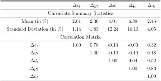
Table 1 first presents summary statistics for log of real, per capita consumption growth, labor income growth, dividend growth, the change in the log of the CRSP price index, ∆pt,
and the change in the log of household net worth, ∆at, all in annual data. Real dividend
growth is considerably more volatile than consumption and labor income, having a standard deviation of 12 percent compared to 1.1 and 1.8 for consumption and labor income growth, respectively. It is somewhat less volatile than the log difference in the CRSP value weighted price index, which has a standard deviation of 16 percent, but still more volatile than the log difference in networth, which has a standard deviation of 4 percent. Consumption growth and labor income growth are strongly positively correlated, as are ∆ptand ∆at. Annual real
consumption growth and real dividend growth have a weak correlation of -0.16.
We begin by testing for both the presence and number of cointegrating relations in the system of variables x′
t ≡ [ct, dt, yt] ′
. Such tests have already been performed for the system
14
v′
t = [ct, at, yt] ′
in Lettau and Ludvigson (2001a) and Lettau and Ludvigson (2002). The results are contained in Appendix C of this paper. We assume all of the variables contained in xtand vtare first order integrated, or I(1), an assumption verified by unit root tests. Test
results presented in the Appendix C suggest the presence of a single cointegrating relation for both vector time series. We denote the single cointegrating relation for v′
t = [ct, at, yt] ′ as α′ = (1, −αd, −αy)′, and for x′t= [ct, dt, yt] ′ as β′ = (1, −βd, −βy) ′ .
The cointegrating parameters αd, αy and βd, βy must be estimated. We use a dynamic
least squares procedure which generates asymptotically optimal estimates (Stock and Watson (1993)).15 This procedure estimates bβ′ = (1, −0.13, −0.68)′
. The Newey-West corrected t-statistics (Newey and West (1987)) for these estimates are -10.49 and -34.82, respectively. We denote the estimated cointegrating residual bβ′xt as ccdyt. The estimated cointegrating
vector for v′
t= [ct, at, yt] ′
isαb′ = (1, −0.29, −0.60)′
, very similar to that obtained in Lettau and Ludvigson (2001a) using quarterly data. The Newey-West corrected t-statistics for these estimates are -14.32 and -30.48, respectively.
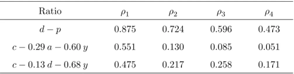
Table 2 displays autocorrelation coefficients for dt− pt, dcayt and ccdyt. It is well-known
that the dividend-price ratio is very persistent. In annual data from 1948 to 2000 it has a first order autocorrelation 0.88, a second order autocorrelation of 0.72 and a third order autocorrelation of 0.60. The autocorrelations of ccdyt and dcayt are much lower and die out
more quickly. Their first order autocorrelation coefficients are 0.48 and 0.55, respectively; their second order autocorrelation coefficients are 0.13 and 0.22 respectively.
In Figure 1 we plot the demeaned values of ccdyt and dcayt over the period 1948 to 2001. The sample correlation between ccdyt and dcayt is 0.41. The figure shows that the two consumption-based present-value relations tend to move together over time, although there are some notable episodes in which they diverge. One such episode is the year 2000, when an extraordinary 30% decline in recorded dividends (an extreme outlier in our sample) pushed ccdyt well above its historical mean.
To better understand the time-series properties of dt− pt, dcayt, and ccdyt, it is useful to
examine estimates of error-correction representations for (dt, pt) ′ , (ct, at, yt) ′ and (ct, dt, yt) ′ . Table 3 presents the results of estimating first-order cointegrated vector autoregressions (VARs) for dt and pt, for ct, at and yt, and for ct, dt, and yt.16 For dividends and prices,
the theoretical cointegrating vector (1, −1)′
is imposed; for the other two systems, the coin-tegrating vectors are estimated as discussed above. The table reveals several noteworthy properties of the data on consumption, household wealth, stock market dividends, and labor income.
First, Panel A shows that the log dividend-price ratio has little ability to forecast future dividend growth or price growth in the cointegrated VAR. Variation in the log dividend-price
15Two leads and lags of the first differences of ∆y
tand ∆dtare used in the dynamic least squares regression. 16The VAR lag lengths were chosen in accordance with findings from Akaike and Schwartz tests. The
ratio is too persistent to display statistical evidence of cointegration in this sample, a result made apparent by the absence of a statistically significant error-correction representation in Panel A (although see the discussion below of the findings in Lewellen (2001) and Campbell and Yogo (2002)). Second, Panel B shows that estimation of the cointegrating residualdcayt−1
is a strong predictor of wealth growth. Both consumption and labor income growth are somewhat predictable by lags of either consumption growth and/or wealth growth, as noted elsewhere (Flavin (1981); Campbell and Mankiw (1989)), but the adjusted R2 statistics
(especially for the labor income equation) are lower than those for the asset regression. More importantly, the cointegrating residualdcayt−1 is an economically and statistically significant determinant of next period’s asset growth, but not next period’s consumption or labor income growth. This finding implies that asset wealth is mean-reverting, and adjusts over long-horizons to match the smoothness of consumption and labor income. These results are consistent with those in Lettau and Ludvigson (2001a) using quarterly data.
Panel C displays estimates from a cointegrated VAR for ct, dt, and yt. The results are
analogous to those for the cointegrated VAR involving ct, at, and yt. Consumption and
labor income are predictable by lagged consumption and wealth growth, but not by the cointegrating residual ccdyt−1. What is strongly predictable by the cointegrating residual is stock market dividend growth: ccdyt−1 is both a statistically significant and economically
important predictor of next year’s dividend growth, ∆dt. These findings imply that when
log dividends deviate from their habitual ratio with log labor income and log consumption, it is dividends, rather than consumption or labor income, that is forecast to slowly adjust until the cointegrating equilibrium is restored. As for asset wealth, dividends are mean reverting and adapt over long-horizons to match the smoothness in consumption and labor income.
4
Long-Horizon Forecasting Regressions
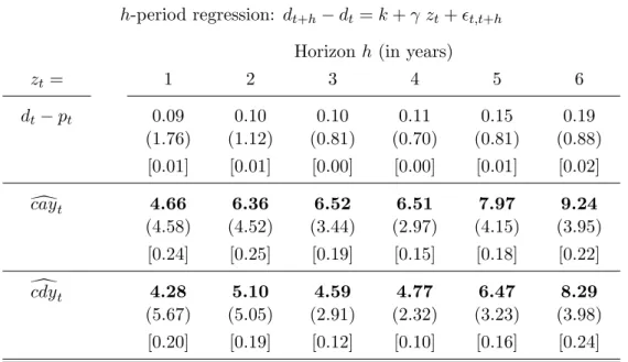
A more direct way to understand mean reversion is to investigate regressions of long-horizon returns and dividend growth onto the consumption ratios ccdyt−1 and dcayt−1. The theory behind (3) and (4) makes clear that both ratios should track longer-term tendencies in asset markets, rather than provide accurate short-term forecasts of booms or crashes. We focus in this paper on explaining the historical behavior of forecastable components of stock market dividend growth, and their relation to forecastable components of excess stock market returns. Table 4 presents the results of univariate regressions of the return on the CRSP value-weighted stock market index in excess of the three-month Treasury bill rate, at horizons ranging from one to 6 years. In each regression, the dependent variable is the H-period log excess return, rt+1 − rf,t+1 + ... + rt+H − rf,t+H, where rf,t is used to denote the Treasury
bill rate, or “risk-freeÔ rate. The independent variable is either dt− pt, dcayt, or ccdyt. The
and a heteroskedasticity and autocorrelation-consistent t-statistic for the hypothesis that the regression coefficient is zero in parentheses. The table also reports, in curly brackets, the rescaled t-statistic recommended by Valkanov (2001) for the hypothesis that the regression coefficient is zero. We discuss this rescaled t-statistic below. Table 5 presents the same output for predicting long-horizon CRSP dividend growth, ∆dt+1+ ... + ∆dt+H. As hinted
at by the results reported in Table 3, neither dcayt, or ccdyt has any important long-horizon
forecasting power for consumption or labor income growth; to conserve space, we do not report those results here.
The first row of Table 4 shows that the log dividend-price ratio has little power for forecast aggregate stock market returns from one to 6 years in this sample. Again, these results differ from those reported elsewhere, primarily because we have included the last few years of stock market data in the sample. The extraordinary increase in stock prices in the late 1990s substantially weakens the statistical evidence for predictability by dt− pt that had
been a feature of previous samples. If we end the sample in 1998, the log dividend price ratio displays forecasting power for excess returns, but its strongest forecasting power is exhibited over horizons that are far longer than that exhibited by the consumption-wealth ratio proxy, d
cayt (see Lettau and Ludvigson (2001a)).17 By contrast, the second row of Table 4 shows
that dcayt has statistically significant forecasting power for future excess returns at horizons
ranging from one to six years. This evidence is consistent with that reported in Lettau and Ludvigson (2001a) using quarterly data. Using this single variable alone achieves an R2 of 0.27 for excess returns at a one-year horizon, 0.49 for excess returns over a two year horizon, and 0.52 for excess returns over a six year horizon.
The remaining row of Table 4 gives an indication of the forecasting power of ccdyt for long-horizon excess returns. At a one year horizon, ccdyt, displays little statistical forecasting power for future returns in this sample. For returns over all longer horizons, however, this present-value relation for dividend growth displays forecasting power for future returns. In addition, the coefficients from these predictive regressions are positive, indicating that a high ccdytforecasts high excess returns just as a high dcaytforecasts high excess returns. The t-statistics are above four for all horizons in excess of one year, and the R2 statistic rises from .20 at a three year horizon to .32 at a six year horizon. Because both caydt and ccdyt are positively related to future excess returns, the results imply that both capture some component of time-varying expected returns.
We now turn to forecasts of long-horizon dividend growth. Table 5 displays results from
17Other statistical approaches find that the dividend-price ratio remains a strong predictor of excess stock
returns even in samples that include recent data. Lewellen (2001) notes that when the dividend-price ratio is very persistent but nonetheless stationary, episodes in which the dividend yield remains deviated from its long-run mean for an extended period of time will not necessarily constitute evidence against predictability. Similar results are reported in recent work by Campbell and Yogo (2002), who find evidence of return predictability by financial ratios if one is willing to rule out an explosive root in the ratios.
the same forecasting exercise for long horizon dividend growth as presented above for long-horizon excess returns. In this sample, which includes data in the last half of the 1990s, the log dividend-price ratio displays some forecasting power for future dividend growth (row 1), but has the wrong sign (positive), consistent with evidence in Campbell (2002) who also uses data that include the second half of the 1990s. Rows 2 and 3 present the results of predictive regressions using dcayt and ccdyt. The consumption-based present value relation for future
dividend growth, ccdyt, has strong forecasting power for future dividend growth at horizons ranging from one to six years. The individual coefficients are highly statistically significant, and the regression results suggest that the variable explains between 20 and 40 percent of future dividend growth, depending on the horizon.
Lettau and Ludvigson (2001a) found that dcayt had predictive power for future returns;
Row 2 shows that it also has statistically significant predictive power for dividend growth rates in our sample, with high values of dcayt predicting high dividend growth rates. The forecasting power of dcayt is, however, weaker than that displayed by ccdyt at every horizon in excess of one year (row 3). For example, at a four year horizon, ccdyt explains about 20 percent of the variation in dividend growth, while dcayt explains 9 percent. At a five
year horizon, ccdyt explains about 28 percent of the variation in dividend growth, while dcayt explains 10 percent. Still, just as for excess returns, the results suggest that both dcayt and
c
cdyt capture some component of time-varying expected dividend growth.
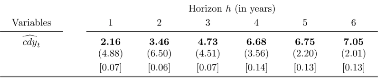
The results in Tables 5 and 6 suggest that there is common variation in expected returns and expected dividend growth. The consumption-wealth ratio proxy,caydt, which is a strong predictor of excess stock market returns, is also a predictor of stock market dividend growth. Conversely, ccdyt, a strong predictor of stock market dividend growth, is also a predictor of
excess stock market returns. A natural question is whether either variable has independent predictive power for excess returns and dividend growth. To address this question, Table 6 presents the results of multivariate regressions of long-horizon excess returns (upper panel) and dividend growth (lower panel) using dcayt and ccdyt as regressors. The table shows that, in forecasting long horizon excess returns, ccdyt contains no information about future returns that is independent of that contained indcayt: at all forecasting horizons,dcayt drives out ccdyt. Even though both variables convey information about future returns and future
dividend growth,dcaytcontains some information about future returns that is independent of that contained in ccdyt. This suggests the presence of an independent component in expected
excess returns, corresponding to the component xt in the discussion above.
The second panel of Table 6 shows that much the opposite pattern is borne out in long-horizon forecasting regressions for dividend growth: ccdytdrives outdcaytin forecasting future dividend growth at all forecasting horizons greater than three years. But for forecasting horizons between 2 and 3 years, the information contained in dcayt and ccdyt is apparently
sufficiently similar that the regression has difficulty distinguishing their independent effects (although ccdyt is statistically significant at the 6 percent level). Accordingly, dcayt and ccdyt
are not marginally significant predictors of dividend growth over 2 and 3 year horizons, but they are strongly jointly significant (the p-value for the F -test is less than 0.000001).
This latter finding suggests that much of the variation in expected dividend growth may be common to variation in expected returns, at least for two and three year horizons. The findings also suggest that there may be a component of expected returns that moves independently of expected dividend growth. Note that if much of the variation in expected dividend growth is common to variation in expected returns, we would not expect innovations in expected dividend growth to have an important effect on the log dividend-price ratio, for the reasons discussed in Section 2. By contrast, if there were a component of expected returns that is independent of expected dividend growth, we would expect innovations in expected returns to have a positive effect on the log dividend-price ratio.
One way to evaluate these possibilities is to estimate elasticities of the dividend-price ratio with respect to innovations in expected dividend growth and expected returns. Such estimates can be accomplished by running regressions of dt− pt on innovations in dcdyt and
d
cayt. The output below is generated by regressing dt− pt on the residuals, εcdy,t and εcay,t,
from first-order autoregressions for dcdyt and caydt, respectively. The lagged log
dividend-ratio is also included as a regressor to control for the substantial persistence in dt− pt. The
estimation output from these regressions using data from 1948 to 2001, with t-statistics in parentheses, is
dt− pt = −0.06
(−1.45) + 0.96(18.89)(dt−1− pt−1) − 1.31(−1.0)εcdy,t
dt− pt = −0.05
(−1.41) + 0.97(22.02)(dt−1− pt−1) + 4.24(2.73)εcay,t.
These results confirm the intuition suggested by the long-horizon forecasting regressions presented above. Innovations in expected dividend growth, as proxied by εcdy,t, have no
sta-tistically significant effect on dt− pt, consistent with the finding that much of the variation
in expected dividend growth is common to variation in expected returns. By contrast, inno-vations in expected returns, as proxied by εcay,t, are statistically significant at conventional
significance levels. These findings reinforce the conclusion that persistent variation in the log dividend-price ratio is better described as capturing some low frequency component of expected excess returns than variation in expected dividend growth, consistent with the ar-guments in Heaton and Lucas (1999), Campbell and Shiller (2001), Cochrane (2001), Fama and French (2002), and Lewellen (2001); Campbell (2002).
4.1
Related Empirical Findings
In summary, the evidence presented above suggests that there is important predictability of dividend growth over long horizons, and that predictable variation in dividend growth is correlated with that in excess returns. To our knowledge, such evidence of important pre-dictability in dividend growth, correlated with important forecastable movements in excess
returns, is largely new. Other researchers, cited in the introduction, have found that divi-dend growth predictability–if evident at all in long-horizon regressions–occurs at relatively short horizons and is not highly correlated with predictable variation in excess returns. More recently, Ang (2002) investigates the forecastability of long-horizon dividend growth for the aggregate stock market using annual data from 1927-2000. Although Ang concludes that there may be some long-horizon forecastability of dividend growth based on results from rolling forward a first-order vector autoregression for dividend yields, dividend growth rates and returns, he finds little evidence of predictability in long-horizon dividend growth from direct long-horizon regressions. These findings are consistent with those of the earlier papers cited in the introduction which use the log dividend-price ratio as a predictive variable, and our own results using dt− pt, reported above.
One recent study that does find predictability of dividend growth in direct long-horizon regressions is Ang and Bekaert (2001), who report results based on observations from 1952:Q4 to 1999:Q4 on the S&P 500 stock market index. Like Ang (2002), they also confirm the earlier findings of Campbell (1991) and Cochrane (1991), that dividend growth is largely unpredictable by the dividend-price ratio in univariate long-horizon forecasting regressions. As Campbell (1991) and Cochrane (1991) emphasize, such findings imply that changing forecasts of future dividend growth must comprise little of the variation in the dividend-price ratio. But, Ang and Bekaert (2001) do find that the dividend-dividend-price ratio has marginal predictive power for future dividend growth in a multivariate regression once the earnings yield is also included as a regressor. (The earnings yield also has marginal predictive power.) There are two main differences between our predictability results and those in Ang and Bekaert (2001). First, the joint forecasting power of the dividend yield and the earnings yield for dividend growth is concentrated at shorter horizons than in regressions using ccdyt and d
cayt. Second, the R-squares for the regressions using the former variables are substantially
lower than those using the latter. For example, in the sample used in Ang and Bekaert (2001), the dividend yield and the earnings yield jointly explain about 21 percent of dividend growth one year ahead, and about 13 percent a five year horizon. The comparable numbers using
c
cdyt alone as a predictive variable are 31 percent and 34 percent.18
4.2
Additional Statistical Tests
4.2.1 Multivariate Long-Horizon Forecasting Regressions19
The cointegrating coefficients in dcayt and ccdyt are estimated using the full sample. This estimation strategy is appropriate for testing the theoretical framework above, because
suf-18These numbers are higher than those reported in Table 4 because we use the slightly shorter sample
employed by Ang and Bekaert (2001) in order to make the results directly comparable.
19We are grateful to Jushan Bai for pointing out the possibility of using the methodology used in this
ficiently large samples of data are necessary to recover the true cointegrating coefficients, and there is no implication (either from the theoretical framework or from statistical theory) that dcayt and ccdyt should forecast the right-hand-side variables in (3) and (4) unless the cointegrating coefficients have converged to their true values. Fortunately, cointegrating co-efficients are “superconsistent,Ô converging to their true values at a rate proportional to the sample size T , and can therefore be treated as known in subsequent estimation. It follows that a valid test of the theoretical cointegration framework in (3) and (4) requires the use of the full sample to estimate the cointegrating coefficients.20
A separate issue concerns not whether the theoretical framework is correct, but whether a practitioner, operating in early part of our sample and without access to the whole sample to estimate cointegrating coefficients, could have exploited the forecasting power of dcayt
and ccdyt. Out-of-sample or subsample analysis is often used to assess questions of this nature. A difficulty with these procedures, however, is that the subsample analysis inherent in out-of-sample forecasting tests entails a loss of information, and can lead such tests to be substantially less powerful than in-sample forecasting tests (Inoue and Kilian (2002)). This means that out-of-sample (and subsample) tests can fail to reveal true forecasting power that even a practitioner could have had in real time. This pattern that would be exacerbated in any investigation of long-horizon forecasting power.
With these considerations in mind, we now provide an alternative approach to assessing the forecasting power of dcayt and ccdyt. The approach we propose eliminates the need to
estimate cointegrating parameters using the full sample in a first stage regression, but at the same time avoids the power problems inherent in out-of-sample and subsample analyses. To do so, we consider single equation, multivariate regressions taking the form
zt+h= a + b1ct+ b2at+ b3yt+ ut, (10)
where the dependent variable zt+h is either the h period excess return on the CRSP
value-weighted index, or the h period dividend growth rate on the CRSP value-value-weighted index. Rather than estimating the cointegrating relation among ct, at, and yt in a first stage
re-gression and then using the cointegrating residual as the single right-hand-side variable, the regression (10) uses the multiple variables involved in the cointegrating relation as regressors directly. If there is a relation between the left-hand-side variable to be forecast, and some stationary linear combination of the regressors ct, at, and yt, the regression can freely
esti-mate the non-zero coefficients b1, b2, and b3 which generate such a relation. For this excercise,
we maintain the hypothesis that the left-side-variable is stationary, while the right-hand-side variables are I (1). Then, under the null hypothesis that (ct, at, yt)
′
has a single cointegrat-ing relation, it is straightforward to show that the limitcointegrat-ing distributions for b1, b2, and b3
will be standard, implying that the forecasting regression (10) will produce valid adjusted
R2 and t-statistics. Because this procedure does not require any first-stage estimation of
cointegrating parameters, it is clear that the forecasting regression (10), its coefficients and R2 statistics, cannot be influenced by such a prior analysis.
Table 6 reports long-horizon regression results for excess returns and dividend growth, from an estimation of (10) and a directly analogous multivariate regression in which ct, dt,
and yt are the regressors. The table reports the coefficient estimates at the top of each cell,
heteroskedasticity and serial correlation robust t-statistics in parentheses, and adjusted R2
statistics in square brackets.21 The results are broadly consistent with those obtained using
d
caytand ccdytas forecasting variables. In almost every case, the individual coefficients on each regressor are strongly statistically significant as predictive variables for excess returns and dividend growth, and the R2 statistics indicate that the regressors jointly explain about the
same fraction of variation in future returns and future dividend growth as do the individual regressors dcayt and ccdyt. For example, the multivariate regression with ct, at, and yt as
regressors explains about 26 percent of one year ahead excess returns, whereasdcayt explains 27 percent. Similarly, the multivariate regression with ct, dt, and ytexplains about 24 percent
of the variation in one-year-ahead dividend growth, whereas ccdytexplains 20 percent. These results do not support the conclusion that dcayt and ccdyt have forecasting power merely because they are estimated in a first stage, using data from the whole sample period. 4.2.2 Small Sample Robustness
There are at least two potential econometric hazards with interpreting the long-horizon regression results using ccdyt and dcay, presented above. One is that the use of overlapping data in long-horizon regressions can skew statistical inference in finite samples. Valkanov (2001) shows that, in finite samples where the forecasting horizon is a nontrivial fraction of the sample size, (i) the t-statistics of long-horizon regression coefficients do not converge to
21Inference on b
1, b2, and b3can be accomplished by re-writing (10) so that the hypotheses to be tested are
written as a restrictions on I (0) variables (Sims, Stock, and Watson (1990)). For example, the hypothesis b1= 0 can be tested by rewriting (10) as
zt+h = a + b1[ct− ωat− (1 − ω) yt] + [b2+ b1ω] at+ [b3+ b1(1 − ω)] yt+ ut
= a + b1[cayt] + [b2+ b1ω] at+ [b3+ b1(1 − ω)] yt+ ut.
It follows that the ordinary least squares estimate of b1 has a limiting distribution given by
√ T°bb1− b1 ± −→ N À 0, σ 2 u TPTt=1(cayt− cay) 2 ! , where σ2
u denotes the variance of ut, and cay is the sample mean of cayt. These may be evaluated by using
the full sample estimates, dcayt. A similar rearrangement can be used to test hypotheses about b2 and b3.
Note that the full sample estimates of the cointegrating coefficients are only required to do inference about the forecasting excercise–they do not affect the forecasting excercise itself.
a well defined distribution, and (ii) the finite-sample distributions of R2 statistics in
long-horizon regressions do not converge to their population values. A second possible econometric hazard with interpreting the long-horizon regression results presented in the previous section occurs because (like most long-horizon forecasting variables) ccdyt and dcay are persistent
variables, which, although predetermined, are not exogenous. This lack of exogeneity can create a small sample bias in the regression coefficient that works in the direction of indicating predictability even where none is present (Nelson and Kim (1993) and Stambaugh (1999)).
To address these potential inference problems, we perform three robustness checks. The first is to compute the rescaled t/√T statistic (where T is the sample size), recommended by Valkanov (2001). Second, we use vector autoregessions to impute long-horizon R2 statistics,
rather than estimating them directly from long-horizon regressions. Third, we perform both bootstrapped and Monte Carlo estimates of the empirical distribution of the predictive regression coefficients and adjusted R2 statistics under the null of no predictability.
We begin by discussing the rescaled t/√T statistic. Valkanov (2001) shows that, when there is nontrivial overlap in the residuals of long-horizon regressions, the t-statistic for whether the predictive variable is statistically different from zero diverges at rate T1/2. Thus,
Valkanov proposes testing for statistical significance by using a rescaled t/√T statistic, which has a well defined limiting distribution. The distribution of this rescaled statistic is nonstandard, however, and depends on two nuisance parameters, δ and c. The parameter δ measures the covariance between innovations in the variable to be forecast, and innovations some forecasting variable, call it Xt. The parameter c measures deviations from unity in the
highest autoregressive root for Xt, in a decreasing (at rate T ) neighborhood of 1. Both of
these parameters may be consistently estimated using the methodology described in Valkanov (2001). With these estimates in hand, the rescaled t-statistic, t/√T , may be compared against critical values provided in Valkanov (2001).
The rescaled t-statistics for our application are reported in curly brackets in Table 4, for univariate predictive regressions of excess returns on dcayt and ccdyt, and in Table 5, for
univariate predictive regressions of dividend growth on dcayt and ccdyt. The table reports both the statistic itself, and whether its value implies that the predictive coefficient in each regression is statistically significant at the 5, 2.5 and 1 percent levels. According to this rescaled t-statistic, dcayt is a powerful forecaster of excess returns (statistically significant at the 1% level) at every horizon ranging from one to six years, as is ccdytat all but the one-year
horizon (Table 4). For future dividend growth (Table 5), the rescaled t-statistic implies that c
cdyt is a statistically significant predictor at the 1% percent level at every horizon from one
to six years, whereas dcayt is a statistically significant predictor of dividend growth at the 1% level at every horizon ranging from one to four years. These results do not support the conclusion that the forecasting power of dcayt and ccdyt for long-horizon excess stock market returns and stock market dividend growth can be attributed to biases arising from the use of overlapping data in finite samples.
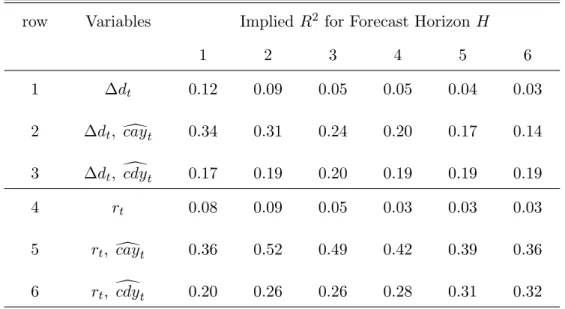
Finite sample problems with overlapping data in long-horizon regressions may also be avoided by using vector autoregression to impute implied long-horizon R2 statistics for
uni-variate forecasting regressions, rather than estimating them directly from long-horizon re-turns. The methodology for measuring long-horizon statistics by estimating a VAR has been covered by Campbell (1991), Hodrick (1992), and Kandel and Stambaugh (1989), and we refer the reader to those articles for further details. We present the results from using this methodology in Table 8, which investigates the long-horizon predictive power of dcayt and
c
cdyt for future returns and future dividend growth using bivariate, first-order VARs. For each forecasting horizon we consider, we calculate an implied R2 statistic using the coefficient
estimates of the VAR and the estimated covariance matrix of the VAR residuals.
Table 8 shows that the pattern of the implied R2statistics from the vector autoregressions
is very similar to those from the produced from the single equation long-horizon regressions. The implied adjusted R2 statistics for forecasting dividend growth with ccdy
t (row 3) peaks
at 0.2 for a three year horizon. This forecasting power is consistently greater than that obtained from a simple autoregression for dividend growth (row 1). A similar pattern holds for the implied R2 statistics for forecasting with dcay
t: the implied R2 statistic for forecasting
excess returns with dcayt is as high as 49% at a three year horizon; for forecasting dividend growth with dcayt, it reaches 24% at a three year horizon. Thus, the evidence favoring
predictability of dividend growth and excess stock returns using ccdyt and dcayt is robust to the VAR methodology, implying that the size of the long-horizon R2 statistics cannot be
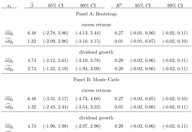
readily attributed to inference problems with the use of overlapping data in finite samples. An alternate method for addressing potential finite sample biases is to estimate the empirical distribution of regression coefficients and adjusted R2 statistics from predictive regressions in which dcaytand ccdyt are used as forecasting variables. Table 9 presents results based on two methodologies which yield very similar results: a bootstrap and a Monte Carlo simulation, both conducted under the null hypothesis of no predictability (i.e., residuals for the dependent variable are generated by regressions on a constant). For both simulations, we use first-order autoregressive specifications our reduced form models fordcayt and ccdyt.22
For the bootstrap, artificial sequences of excess returns and dividend growth are generated by drawing randomly (with replacement) from the sample residuals, under the null of no pre-dictability.23 The simulations were repeated 10,000 times. For the Monte Carlo simulation,
10,000 artificial time-series equal to the size of our data set were generated under the null of no predictability by taking random draws from a normal distribution; the notes to Table
22It is known that the standard bootstrap is not consistent if the data series have a near-unit root.
However, dcayt and dcdyt do not appear well-characterized as near-unit root processes, since—unlike the log
dividend-price ratio—standard cointegration tests strongly reject the hypothesis that they are I (1) random variables.
23Nelson and Kim (1993) also perform randomization, which differs from bootstrapping only in that
sampling is without replacement. We also performed the simulations using randomization and found that the results were not affected by this change.
9 provides details. To avoid difficulties caused by the use of overlapping data, we focus here on the one-year ahead regressions presented in Tables 5 and 6.
Table 9 summarizes the estimated sampling distribution for the slope coefficient and the R2statistic in univariate forecasting regressions of annual excess returns and annual dividend
growth. Panel A presents the bootstrap results; Panel B, the Monte Carlo results. The results of each simulation are nearly identical. In almost every case, the estimated predictability coefficient and R2 statistic lies outside of the 95 percent confidence interval based on the
empirical distribution under the null of no predictability. In most cases they lie outside of the 99 percent confidence interval. The one exception is for the case in which excess returns are regressed on the one-year lagged value of ccdy; in this case, we cannot reject the hypothesis that one-step ahead forecasting power of ccdyt is not statistically indistinguishable from zero.
This is not surprising, since even the standard asymptotic statistics suggest that ccdytonly has significant predictive power for returns at horizons longer than one year. For all of the other regressions and forecasting horizons, we find that our estimated slope coefficients and R2
statistics are large relative to their sampling distributions under the null of no predictability. In summary, these results, like those discussed above using the rescaled t-statistic and VAR-imputed R2 statistics, do not support the conclusion that the predictability of excess returns
and dividend growth documented here is can be attributed to small sample biases in the regression coefficients or R2 statistics.
4.3
Including Share Repurchases
So far we have focused on measuring dividends as the actual cash paid to shareholders of the CRSP value-weighted index. We do this in order to make our results directly comparable with the existing literature which has focused on forecasting the growth rate in this particular measure of dividends. This measure is of interest because it represents the predominant form of payout to shareholders over much of the post-war period. Moreover, as noted by Campbell and Shiller (2001), traditional dividends are an appealing indicator of fundamental value for long-term shareholders, because the end-of-period share price becomes trivially small when discounted from the end to the beginning of a long holding period.
Nonetheless, there is a growing view that changing corporate finance policy has led many firms, in recent years, to compensate shareholders through repurchase programs rather than through dividends (Fama and French (2001); Grullon and Michaely (2002)), even if large firms with high earnings have continued to increase traditional dividend payouts over time (DeAngelo, DeAngelo, and Skinner (2002)). In this section we show that our main conclusions are not altered by adjusting dividends to account for share repurchase activity.
One way to adjust dividends for such shifts in corporate financial policy is to add dollars spent on repurchases to dividends. We do so here by adding aggregate share repurchase expenditures for the Industrial Compustat firms reported in Grullon and Michaely (2002)