Survey and Proposal of an Adaptive Anomaly Detection Algorithm for Periodic Data Streams

ISSN Print: 2327-5219

DOI: 10.4236/jcc.2019.78004 Aug. 29, 2019 33 Journal of Computer and Communications

Survey and Proposal of an Adaptive Anomaly

Detection Algorithm for Periodic Data Streams

Zirije Hasani, Samedin Krrabaj

Faculty of Computer Science, University “Ukshin Hoti”, Prizren, Kosovo

Abstract

Real-time anomaly detection of massive data streams is an important research topic nowadays due to the fact that a lot of data is generated in continuous temporal processes. There is a broad research area, covering mathematical, statistical, information theory methodologies for anomaly detection. It ad-dresses various problems in a lot of domains such as health, education, finance, government, etc. In this paper, we analyze the state-of-the-art of data streams anomaly detection techniques and algorithms for anomaly detection in data streams (time series data). Critically surveying the techniques’ per-formances under the challenge of real-time anomaly detection of massive high-velocity streams, we conclude that the modeling of the normal behavior of the stream is a suitable approach. We evaluate Holt-Winters (HW), Tay-lor’s Double Holt-Winters (TDHW), Hierarchical temporal memory (HTM), Moving Average (MA), Autoregressive integrated moving average (ARIMA) forecasting models, etc. Holt-Winters (HW) and Taylor’s Double Holt-Winters (TDHW) forecasting models are used to predict the normal behavior of the periodic streams, and to detect anomalies when the deviations of observed and predicted values exceeded some predefined measures. In this work, we propose an enhancement of this approach and give a short description about the algorithms and then they are categorized by type of prediction as: predic-tive and non-predicpredic-tive algorithms. We implement the Genetic Algorithm (GA) to periodically optimize HW and TDHW smoothing parameters in ad-dition to the two sliding windows parameters that improve Hyndman’s MASE measure of deviation, and value of the threshold parameter that de-fines no anomaly confidence interval [1]. We also propose a new optimiza-tion funcoptimiza-tion based on the input training datasets with the annotated anoma-ly intervals, in order to detect the right anomalies and minimize the number of false ones. The proposed method is evaluated on the known anomaly de-tection benchmarks NUMENTA and Yahoo datasets with annotated anoma-lies and real log data generated by the National education information system How to cite this paper: Hasani, Z. and

Krrabaj, S. (2019) Survey and Proposal of an Adaptive Anomaly Detection Algorithm for Periodic Data Streams. Journal of Computer and Communications, 7, 33-55.

https://doi.org/10.4236/jcc.2019.78004

Received: July 10, 2019 Accepted: August 26, 2019 Published: August 29, 2019

Copyright © 2019 by author(s) and Scientific Research Publishing Inc. This work is licensed under the Creative Commons Attribution International License (CC BY 4.0).

http://creativecommons.org/licenses/by/4.0/

DOI: 10.4236/jcc.2019.78004 34 Journal of Computer and Communications (NEIS)1 _{in Macedonia.}

Keywords

Anomaly Detection, Periodic Time Series, HOLT Winters Algorithm, Genetic Algorithm GA, MASE, HTM

1. Introduction

Anomaly detection in real-time massive data streams (practically infinite flow of data, pouring in as time goes, each piece of data having its own timestamp) is one of the important research topics nowadays due to the fact that the most of the world data generation is a continuous temporal process. Many sophisti-cated and highly effective anomaly detection methods exist that run-in batch mode, where the data is collected and processed after the occurrence. Howev-er, identifying anomalies long after they happened isn’t our primary goal. On the contrary, real-time data processing, requests continual input, time-critical manner processing, and instant output (e.g. alarm) if anomaly happened. In-stead of searching for the unknown anomalies we can, in advance, model a normal behavior of the data stream and compare it to the observed one. Con-sequently, predicting the values of a stream one-time step ahead are used, the deviation between the predicted values and the observed values are measured, and a decision mechanism, if an observed value exceeds normal behavior, is established. Yet other questions arise. The real-time streams are infinite, can have a high rate of data appearance in time unite (high volume, high velocity) and can evolve over time. Thus, the development of the model of normal be-havior must adapt to these challenges to maintain detection accuracy: be itera-tive, use only a part of the stream (even before it is permanently stored), and be implemented as a positive feedback in the learning process (e.g. repeated anomalies labeling in the supervised process). Due to the need for the real-time detection process, detection algorithms have to be robust, with low processing time (low complexity), even at the cost of the accuracy. Currently, the most intensively developed anomaly detection methods that consider un-derlined challenges are based on machine learning, neural networks, predictive and statistical time series forecasting models.

In this paper, we are interested in anomaly detection of real data streams that have seasonal patterns. There are a number of studies in this area. The most adequate and often used models are Moving Average (MA) [2], the AutoRegres-sive Moving Average (ARMA) and AutoRegresAutoRegres-sive Integrated Moving Average (ARIMA) [2], exponential smoothing algorithms HW [3] and TDHW [4], Hie-rarchical Temporal Memory (HTM) [5] algorithm and sliding windows [6] [7].

However, our work brings several benefits [1]:

DOI: 10.4236/jcc.2019.78004 35 Journal of Computer and Communications • _{From all the reviewed literature for anomaly detection, we assessed methods}

and algorithms for anomaly detection in data streams (time series) which are proper and capable to respond to the challenges that massive data streams and real-time detection have;

• _{We propose an enhancement of the additive HW and TDHW algorithms} that answers the stated challenges. The algorithm is implemented as a posi-tive feedback optimization with a periodic adaptation of the algorithm para-meters;

• Starting with ideas of numerous papers [4] [7]-[13], we use the GA optimiza-tion process, to optimize α, β, γ, ω, the HW and TDHW smoothing parame-ters, where we added optimization of the three new parameters k, n and δ; • _{Improvement is made in the new definition of the optimization function}

based on the input training datasets with the annotated anomaly intervals, enhanced Hyndman’s MASE [14] definition where k and n define the two sliding windows intervals, and δ is the threshold parameter;

• _{The positive feedback learning process is achieved if the anomalies detected} in the next time frame, by the proposed detection engine based on the com-puted optimal parameters from the annotated anomalies of previous one, are verified/acknowledged by human and reused for parameter optimization; • _{The results of the experiments performed on the sets of synthetic and real data}

periodic streams show that our proposed HW algorithm, with GA optimized parameters and with improved MASE, outperforms the other algorithms. The data used for experiments are known as anomaly detection benchmarks NUMENTA [12] and Yahoo [15] datasets with annotated anomalies and our real log data from the Macedonian national education system e-dnevnik1_.

The rest of this paper has the following structure: in the second section is re-lated work; in the third section proposed a model for real-time data streams anomaly detection is described, in the fourth section are the experimental re-sults; and the last section contains conclusions and further work.

2. Review and Classification of Methods for Anomaly

Detection

In this section, we have shown some algorithms used for anomaly detection clas-sified by type of data, type of anomalies, application area, type of supervision and also is done classification of algorithms as predictive and non-predictive.

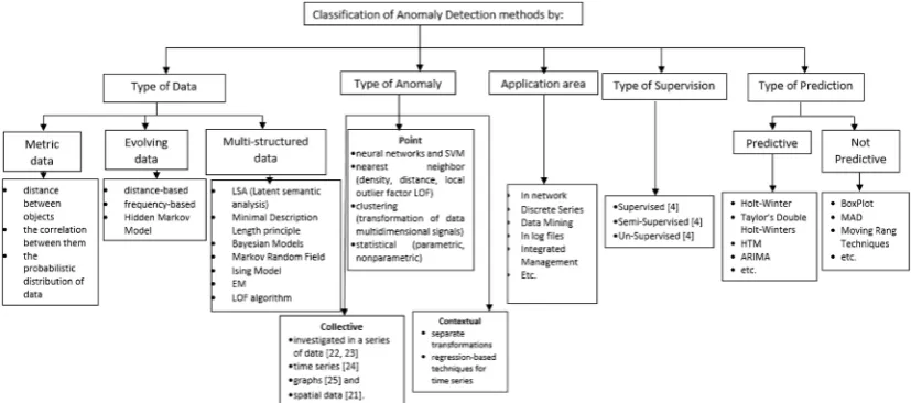
In Figure 1 below is shown the classification which is done for anomaly

de-tection algorithms for different fields.

2.1. Classification of Anomaly Detection Methods by Type of Data

Kalinichenko et al., 2014 [2] categorize the data (and related methods) into three categories: the metric data, evolving data, and multi-structured data.

The Metric Data

DOI: 10.4236/jcc.2019.78004 36 Journal of Computer and Communications

Figure 1. Classification of anomaly detection methods.

them, and the probabilistic distribution of data. Further subdivision is based on the notion of distance (clustering methods, K nearest neighbors and their deriv-atives), based on the correlations (method of linear regression, PCA-Principal component analysis), data distributions, an iterative algorithm based on the maximum likelihood method, and methods related to the data with high dimen-sion (methods of dimendimen-sionality reduction).

The Evolving Data (Discrete Sequences Data and Time Series Data) The methods for Discrete Sequences Data are distance-based, frequency-based and Hidden Markov Model that measure the deviation of a specific value or whole sequence. In the survey [1], the methods are divided into three groups: sequence-based, contiguous subsequence-based and pattern-based. The first group includes Kernel Based Techniques, Window Based Techniques, Marko-vian Techniques, contiguous subsequence methods include Window Scoring Techniques and Segmentation Based Techniques. Pattern-based methods in-clude Substring Matching, Subsequence Matching, and Permutation Matching Techniques. For the category of Time series data, the methods that are used are based on well-developed apparatus of time series analysis, including predictive methods, Kalman Filtering, Autoregressive Modeling, detection of unusual shapes with the Haar transform and various statistic techniques.

Multi-Structured Data

The data are categorized into two categories: text data and graph data. The methods used for outlier detection in text data are LSA (Latent semantic analy-sis) which makes it possible to group text, integrating it with the standard ano-maly detection methods, and tf-idf measure. For graph data, the methods are Minimal Description Length principle, Bayesian Models, Markov Random Field, Ising Model, EM and LOF algorithm.

2.2. Classification of Methods by Type of Anomalies

DOI: 10.4236/jcc.2019.78004 37 Journal of Computer and Communications and Pokrajac et al., 2008 [16] classify methodologies according to the type of anomaly (point, contextual, and collective anomaly).

The widest range of methodologies is devoted to the simplest one, a point ano-maly detection. These are classification methodologies, supervised, semi-supervised and unsupervised (based on the rules, neural networks and SVM), methodolo-gies based on the nearest neighbor (density, distance, local outlier factor LOF), clustering (transformation of data multidimensional signals), statistical (para-metric, nonparametric) methods based on the information theory, and statistical probability, spectral-based visualization and others. Contextual anomalies (also called conditional anomalies’2_{). Often occur in data such as time series [17] [18],} and spatial data [19] and the choice of the methodologies is often associated with the application domain. Unlike point anomalies, for the contextual anomalies, there is not a wide range proposed methodology. They fall into two categories: using separate transformations to reduce the problem into a point anomaly de-tection in a particular context, for example, the methodology illustrated in the

[20] and predictive sequence and time series in methodologies (mostly regres-sion-based techniques for time series).

The collective anomaly occurs when the collection of instances deviates in re-lation to other data. For example, an individual event in the computer system does not necessarily mean anomaly, but a certain sequence of events can mean a hacker attack. The collective anomaly may exist if the data are associated with certain relations. It is investigated in a series of data [21] [22], time series [23], graphs [24] and spatial data [19]. The discovery of collective anomalies is more complex in terms of point and contextual anomalies since it requires a separate examination of the structure.

2.3. Classification of Methods by Application Area

Due to the wide number of areas for anomaly detection, the authors of some comparative studies limited themselves to the comparison of methods and techniques of detection of anomalies by a separate research field, data type or application area. Thus Phua et al. 2004 [25], Dua and Du [26] Sreevidya et al.,

2014 [27], compare methods in the field of data mining, Chandola et al., 2009

DOI: 10.4236/jcc.2019.78004 38 Journal of Computer and Communications terms of the application field, the type of anomaly, the data characteristics, and computational complexity.

2.4. Classification of Methods by Type of Supervision

The other significant classification of methods is by type of supervision. A training data set is required by techniques which involve building an explicit predictive model. The labels associated with a data instance denote if that in-stance is normal or an outlier. Based on the extent to which these labels are uti-lized Chandola et al., 2009 [1], outlier detection techniques divide into the three categories: supervised, semi-supervised and unsupervised outlier detection tech-niques.

2.5. Review of Predictive and Not Predictive Algorithms for

Real-Time Anomaly Detection in Massive Data Streams

(Contextual Anomalies)

Usually, authors of newly proposed algorithms for anomaly detection compare their results with the results of the state-of-the-art techniques (for example, LOF, k-NN), but often, they do not take into account a possibility of real-time detec-tion in a huge amount of incoming data. The starting goal of this work was to evaluate different categories of algorithms, (we divided them into predictive and non-predictive (statistical) algorithms), for which we expected to be fast and with satisfactory detection rate (sensitivity-recall and precision [32] [33]) and so suitable for real-time anomaly detection of massive data streams.

Several algorithms were explored, MAD, runMAD [34], Boxplot [35], Twitter ADVec [36], DBSCAN [37] [38], our proposal combination of runMAD and Boxplot, ARIMA [39], Moving Range Technique [40] [41], Statistical Control Chart Techniques [39], Moving Average [42], Hierarchical Temporal Memory (HTM), Holt-Winters and Taylor’s Double Seasonality Holt-Winters.

Autoregressive (AR) and Moving Average (MA) forecasting models have been in existence since the early 1900s. Exponential Smoothing Methods, as a forecasting tool, are introduced in the 1950s. Detailed history, statistical theory, and classification depending on the time series characteristics can be found in [43].

Following is a more detailed review of the research papers dealing with Holt-Winters and Taylor’s Double Seasonality Holt-Winters forecast modeling of normal data streams behavior. Papers are grouped in studies where HW and TDHW models are used for anomaly detection and their model parameters cal-culated by exponential formula or decided experimentally [3] [44] [45], studies that deal with optimization of the model parameters for the best fitted forecast

[4] [8] [9] [10] [46], parameter optimization are done using classical

DOI: 10.4236/jcc.2019.78004 39 Journal of Computer and Communications J. Brutlag [44] for the first time in the 2000 year, used a model based on HW forecasting. He integrated it into the Cricket/RRDtool open source monitoring tools to detect automatically, in the real-time, aberrant behavior of the WebTV services streams. He proposed usage of the exponential formulas for calculation of the smoothing parameters. The anomaly is detected if the new observed data stream value yt falls outside the interval, determined by the measure of deviation dt for each time point in the seasonal cycle. Deviation dt is a weighted average of absolute deviation, updated via exponential smoothing (calculated with the same parameter γ as a sessional factor in HW). While perhaps not optimal, this solu-tion was shown as a flexible, efficient, and effective tool for automatic detecsolu-tion. Authors in [3] implement the same idea in multiplicative HW forecasting mod-el, as a part of a test platform that collects real IP flow, based on open source software Nfsen/RRDtool. Calculation of the parameters was as in [44]. They used Mean Absolute Error (MAE) and Root Mean Square Error (RMSE) as suitable to compare different forecasting methods and Mean Absolute Percen-tage Error (MAPE), to compare how a forecasting method suits forecasting dif-ferent time series. In [45] author emphases the need of close examination of the stream behavior before choosing the forecast model: trend existence, characteri-zation of single/multiple seasons, threshold determination concerning the im-portance of a number of correct and false detections, and a number of detected anomalies in time unit to signal an alarm.

Optimization of parameters in forecasting model is dating back to 1996 [8]. GA optimization is applied to determine HW smoothing parameters α, β, γ, in-cluding variable s, a seasonality interval, and corresponding start-up values for level, trend, and seasonality, by minimizing the evaluation function forecasting Mean Square Error (MSE). As the forecasting task presented in this thesis did not require a great precision for the parameters and the start-up values, a binary GA (not a real-valued one) is used. Authors underline the great applicability of GA in such type of prediction tasks, especially when a large number of parame-ters is required.

Similarly to the previous paper, in the [46], optimization of HW parameters are done along with tuning of the GA initialization, population size, and cros-sover probability, that enable the comparative study of the best accuracy predic-tion (minimum value) of MAPE. The data used in this study are monthly data set for the total number of tourist arrivals in the ten years period.

DOI: 10.4236/jcc.2019.78004 40 Journal of Computer and Communications In Ashraf [4] authors improved prediction accuracy MSE by employing Ar-tificial Bee Colony algorithm to optimize smoothing parameters of the multip-licative multi sessional HW forecasting model. Cloud workload with mul-ti-seasonal cycle’s data stream is forecasted to scale in advance computational resources. Performance of the proposed algorithm has been evaluated with double and triple exponential smoothing methods using MAPE and RMSE.

In [9] authors optimize α, β, γ, δ, smoothing parameters, φ damped parameter and λ adjustment for the first-order autocorrelation error, of the multiplicative double seasonality and additive damped trend forecast HW. They compare the results of minimization of the sum of squared errors equation (SSE) by several meta-heuristic methods: local improved procedure HC and SA, Evolutionary Algorithms (EA), GA, PS. Optimization is implemented in MATLAB for Portu-guese three months electricity demand stream of data. The conclusion is that the values obtained for the forecasting equation’s parameters using different me-ta-heuristic algorithms were similar as well as the post-sample forecasting per-formance which suggests that HC algorithm for its simplicity is a good solution.

In [10] authors use PS metaheuristic minimizing the Residual Standard Error

(RSE), Sum of Squared Errors (SSE), Mean of Squared Errors (MSE) or Mean Absolute Deviation (MAD) to determine optimal smoothing parameters of the additive Holt model. The direction of the exchange rate and the actual exchange rate values for the Dollar-Peso and Euro-Peso is accurately forecasted.

In [7] work is interesting due to proposed ideas of optimization of the sliding time windows that defines set of time legs used to build various forecasting me-thods and also define the number of the model inputs, using the Genetic and Evolutionary Algorithms (GEA) with a real-valued representative.

Ideas for using metaheuristic optimization of parameters of similar forecast-ing models exist. In [49], Seasonal Autoregressive Integrated Moving Average SARIMA forecasting model parameters are optimized by GA. In [11], authors compared slightly modified HW (that instead of using the time intervals imme-diately before the analyzed ones for the forecasting calculation, used the time in-tervals that are equal to the current and relating to the prior seasonal cycle), with the Ant Colony Optimization (ACO) cluster model.

For more details about the suitable algorithms and their classification are giv-en in the following section.

3. Methods

Next are presented the algorithms which are used to compare the proposed me-thod and are shown the proposed meme-thod [1].

3.1. Algorithms for Anomaly Detection in Real-Time Massive Data

Streams

DOI: 10.4236/jcc.2019.78004 41 Journal of Computer and Communications robust with low processing time, eventually at the cost of the accuracy.

The studied algorithms we categorize into two classes: 1) Non-predictive, statistical (Boxplot, DBSCAN, MAD); 2) Predictive (HTM, ARIMA, HW, TDHW).

We choose to analyze algorithms with rather low computational complexity runMAD [34], Twitter ADVec [36], Boxplot [35], Moving range technique [40] [41], Statistical Control Charts [39], ARIMA [39], Moving Average [42], DBSCAN [37] [38], HTM [5], HW [45] and TDHW [43]. All of them we im-plement in R language [50] except HTM, which is already implemented in NAB environment [12].

DBSCAN algorithm is a density-based clustering algorithm. It works by gree-dily agglomerating points that are close to each other. Outliers are considered clusters with few points in them [38]. This algorithm has two main parts: a pa-rameter ε that specifies a distance threshold under which two points are consi-dered to be close; and the minimum number of points that have to be within a point’s ε-radius before that point can start agglomerating.

The Tukey (1977) BoxPlot does not make any distribution assumptions nor does it depend on a mean or standard deviation. The lower quartile (q1-the 25th percentile), and the upper quartile (q3-the 75th percentile) of the data define the inter-quartile range (IQR) and lines (whiskers) are indicating variability outside the upper and lower limits (9th and 91st percentile or 1.5 IQR over and below IQR defining anomalies.

RunMAD3 _{(Median Absolute Deviation of Moving Windows) for streaming} data is the median of the absolute deviations from the data’s median for the de-fined window. As such does not make any distribution assumptions. Similar window functions are runmin, runmax, runmed, runquartile, etc. Depending on the stringency of the researcher’s criteria, which should be defined and justified by the researcher, the author [51] proposes the values of k = 3 (very conserva-tive), k = 2.5 (moderate conservative) or even k = 2 (poor conservative) for anomaly detection that are outside Median ± k*MAD.

Twitter ADVec [36] proposed by Twitter is composed of different algo-rithms. The primary algorithm, Seasonal Hybrid ESD (S-H-ESD), builds upon the Generalized ESD test for detecting anomalies. S-H-ESD can be used to detect both global and local anomalies. This is achieved by employing time se-ries decomposition and using robust statistical metrics, viz., median together with ESD. In addition, for long time series such as 6 months of minute data, the algorithm employs piecewise approximation. This is rooted in the fact that trend extraction in the presence of anomalies is non-trivial for anomaly detec-tion.

DOI: 10.4236/jcc.2019.78004 42 Journal of Computer and Communications limits are chosen so that almost all the data points will fall within these limits as long as the process remains in control. Data could be a chart of individual data, aggregated by a time parameter (e.g. hour), moving range, moving average and others.

In statistics and econometrics, and in particular in time series analysis, an autoregressive integrated moving average (ARIMA) model is a generalization of an autoregressive moving average (ARMA) model. Both of these models are fitted to time series data either to better understand the data or to predict fu-ture points in the series (forecasting) Moving average. In time series analysis, the moving average (MA) model is a common approach for modeling univa-riate time series. Together with the autoregressive (AR) model, the mov-ing-average model is a special case and key component of the more general ARMA and ARIMA models of time series, which have a more complicated stochastic structure.

Hierarchical Temporal Memory (HTM) [5] is a machine learning algorithm based on the input stream and prediction of the next value. Raw anomaly score that measures the deviation between the model’s predicted input and the actual input is calculated. The distribution is modeled as a rolling normal distribution where the sample mean and variance are continuously updated from previous anomaly scores. The recent short-term average of anomaly scores is using to ap-ply as mean to the Gaussian tail probability to decide whether to declare an anomaly. HTM can robustly detect anomalies in a variety of conditions. The re-sulting system is efficient, extremely tolerant to noisy data, continually adapts to changes in the statistics of the data, and detects very subtle anomalies while mi-nimizing false positives.

3.2. The Adaptive Algorithm for Anomaly Detection

In Figure 2, the positive feedback optimization method for continuous

adapta-tion of the anomaly detecadapta-tion parameters is shown. The method is composed of four different stages [1].

DOI: 10.4236/jcc.2019.78004 43 Journal of Computer and Communications First is the annotation of the anomalies in the training dataset. The anomaly annotation is defined as a time interval where an anomaly is located. The anno-tation is done by a human or an oracle.

The second stage is the computation of anomaly detection parameters for our algorithm using GAs, i.e. computation of HW or TDHW parameters, together with δ, k and n. GAs have been successfully applied to solve optimization prob-lems, both for continuous (whether differentiable or not) and discrete functions”

[14]. This enables us to find near-optimal values of the anomaly detection para-meters very successfully.

The third stage is the actual anomaly detection engine based on the computed optimal parameters from the second stage. This stage outputs the detected ano-malies with our proposed algorithm.

The fourth stage is the human acknowledgment of the output data, and clas-sifies the output data into TP (true positive), FP (false positive) and FN (false negative). The result of the verification/acknowledgment stage is then used again in the second stage for further optimization of the anomaly detection parameters.

In the rest of this section, we present the improved algorithm for anomaly de-tection of real data streams with sessional patterns, based on well-known HW and TDHW [3] [4] additive forecasting models.

The first improvement is done by modification of the Mean Absolute Scaled Error (MASE) [52], and the second one by optimization of the model parame-ters.

3.2.1. Standard Algorithms for Anomaly Detection and MASE Modification

Additive HW trend forecast prediction yˆt+1 is defined iteratively (1) by three components, level lt, trend bt and seasonality st using restricted real smoothing constants 0 ≤ α, β, γ ≤ 1:

Forecast equation: yˆt+1 = + +l b st t t m− +1 Level: lt=α

(

) (

)(

)

(

) (

)

t t t t

b =β l l− − + −β b− (1)

Seasonality: st =γ

(

) (

)

where m is the periodicity of the one whole seasonal cycle, i.e. the number of time steps of one season. Good initial values l0,b0 and s0 (2) can be achieved by having yt streaming data of two full sessional cycles 2m.

Initial level component: 1 2

0 y y . ym

l

m

+ +… +

=

Initial trend component: 2

1 1

0 2

m m

t t

t m y t y

b

m

= + − =

=

∑

∑

DOI: 10.4236/jcc.2019.78004 44 Journal of Computer and Communications Additive TDHW, trend forecast prediction yˆt+1 (3) is defined iteratively by four components: level lt, trend bt, m1 seasonality and m2 seasonality, using re-stricted real smoothing constants 0 ≤ α, β, γ, ω ≤ 1.

Forecast equation: yˆt+1= + +l b Dt t t+Wt

Level: lt =α

(

)

(

)(

)

(

) (

)

t t t t

b =β l l− − + −β b− (3) m1 seasonality: Dt =γ

(

)

(

)

m2 seasonality: Wt=ω

(

)

(

)

For example, if the stream values yt are observed every minute a daily cycle m1 = 24 × 60 = 1440 and a weekly cycle m2 = 24 × 60 × 7 = 10,080 [53]. Possible initial values are:

0 1 l = y

0 0 b =

1

0,1 0,2 0,m 0 D =D ==D =

2

0,1 0,2 0,m 0 W =W ==W =

Measurement of the forecast accuracy (by using MASE), defined by Hynde-man [52] is calculated as follows:

1 2 ˆ 1 1 t t t _l i i i y y q y y

l = −

− = − −

∑

MASE t i

i q

t =

=

_∑

where l is a number of values in the training stream. In the anomaly detection models based on HW or TDHW models [3] [44] [53], if MASE > δ, where δ is a predefined threshold, the new arrived stream data yt is determined as an anomaly.

We propose [1] an adoption of the MASE definition (5) by adding two win-dow parameters k and n, to the current iterative processes (1) and (3) with smoothing parameters α, β, γ and ω. For the HW forecast, MASE depends on parameters α, β, γ, δ, k, n and for TDHW, MASE depends on parameters α, β, γ, δ, k, n.

( , , , ,) 1 ˆ 1 k t t

t _{t k}

i i i t y y q y y k

α β γ δ ₋

− = − = −

∑

t _{t k}

i i i t y y q y y k

α β γ ω δ ₋

− =

− =

−

∑

where k t< _.

( , , , , ,) ( , , ,, , ,)

1

MASEtα β γ δ_{k n n} t ni tqiα β γ δ_{k n}

− =

=

∑

, , , , , , , , , , , ,

1

MASEtα β γ ω δ_{k n n} t ni t qiα β γ ω δ_{k n}

− =

=

∑

where n t< .

DOI: 10.4236/jcc.2019.78004 45 Journal of Computer and Communications 3.2.2. Finding the Optimal Values of the Algorithm Parameters

The goal of our proposed algorithm is to find the optimal parameter values for the anomaly detection algorithm in order to achieve the correct TP and zero FP and FN.

The evaluation of the optimization parameters for the anomaly detection is based on input datasets and annotated anomaly intervals. We define the follow-ing procedures for countfollow-ing the TP, FP and FN:

• _{TP (true positive) is the number of anomalies annotated intervals with at} least one detected anomaly;

• FP (false positive) is the number of detected anomalies outside of all anno-tated intervals;

• _{FN (false negative) in the number of annotated intervals with 0 detected} anomalies.

Having defined these values, we use the following evaluation function for our genetic algorithm optimization:

( , , , , , , , , , ,1 2 3 4) 1 2 3 4

EFα β γ ω δ_{k n w w w w} =TP∗w −FP∗w −FN∗w − ∗

δ

where w1, w2, w3 and w4 are weight factors (constants) that are given based on the importance of the targeted goals. In our case, we favor to achieve correct TP, and minimal FP and FN, hence the w1 is 100 and w2, w3 and w4 are 1.

Based on the defined EF (6), we use a real-valued GA optimization for para-meters optimization using the following constraints:

0< ≤α 1 0≤β γ ω, , ≤1

max

0< <δ δ

0<n k, ≤ ∗2 m

EF starts with a calculation of a prediction using additive HW (1). Then based on this prediction, we calculate MASEt (4) and evaluate its value against δ. δmax is defined experimental based on the dataset (in our case 50). If our algo-rithm detects an anomaly, we add the timestamp to a list of anomalies for fur-ther evaluation. The next step is an evaluation of the anomaly list against the anomaly annotated intervals, thus deriving TP, FP and FN, and finally calculat-ing the EF value.

The GA optimization is very effective: we use small populations with less than 100 individuals, and achieve the optimal solutions in less than 20 iterations. The proposed algorithm is implemented in R language.

4. Experimental Results

DOI: 10.4236/jcc.2019.78004 46 Journal of Computer and Communications

4.1. Experimental Datasets

To evaluate the proposed algorithm, we have used the most known benchmarks from Yahoo, Webscope dataset “data-labeled-time-series-anomalies-v1_0” [15],

NAB [12] “artificial With Anomaly” and our real data log-file, generated by

NEIS.

We have exploited the first 4 out of 100 Yahoo synthetic A2 and real A3 and A4 time-series benchmarks, with tagged anomaly points. The datasets are suitable for testing the detection accuracy of various anomaly-types including outliers and change-points. The synthetic dataset consists of time-series with the varying trend, noise and seasonality, while the real one consists of time-series representing the metrics of various Yahoo services. Some datasets have a weekly and some a weekly and daily seasonality Part of the datasets A4 is shown in Fig-ure 3 below.

NAB contains artificially-generated datasets with varying types of tagged anomalies and a daily seasonality. The NEIS dataset has weekly and daily seaso-nality. Anomalies are unknown but are analyzed and tagged by a human. All the datasets contain a timestamp and single value based on the log.

4.2. Results and Discussion

In order to evaluate if the optimization of the parameters works well, we have separated the datasets into training and test sets. The optimal values of the pa-rameters are determined on the training set and then they are verified on the test set.

Our proposed algorithm (HW GA) with GA optimized parameters (α, β, γ, δ, k, n) and with improved MASEt₍α β γ δ_{, , , , ,k n)} is compared with ARIMA, MA

(im-plemented in our previous work [54]), HTM [5] algorithm,

HW where smoothing parameters are calculated by formula and default MASE (HW calc. MASE), HW by default smoothing parameters (optimized in R) and default MASE (HW def. MASE), HW by default smoothing parameters and improved MASEk n, (HW def. MASE(k, n)).

DOI: 10.4236/jcc.2019.78004 47 Journal of Computer and Communications HW GA [1] counts automatically the number of TP, FP and FN that is not possible with other compared algorithms. The smoothing parameters can be calculated by Formula (7) were for the total weight we take 0.95:

(

)

log 1 total weights as% 1 exp

# of time points

α = −  − 

  (7)

A number of points (frequency) for Yahoo benchmark stream, with week seasonality, is 24 × 7 = 168, having data each hour. A number of points for the Numenta benchmark stream are 12 × 24 = 288 having data every 5 minutes.

To be able to compare the results we use detection rate (recall) in % (d.r.) and precision (prec.), the statistical performance measures of a binary classification test. Due to the big number of the TN-True Negative values, specificity (the true negative rate) and accuracy are not applicable measures for the time series data.

In Tables 1-5 below, a number of detected TP, FP and FN for NUMENTA,

Yahoo, and NEIS on training and test sets are given.

Similarly, the Taylor’s Double Holt Winters GA (TDHA GA) with optimized parameters (α, β, γ, ω, δ, k, n) and with improved MASEt₍α β γ δ_{, , ,, , ,k n)}, is compared

with the same algorithms as for HW, where HW type algorithms are replaced with TDHW.

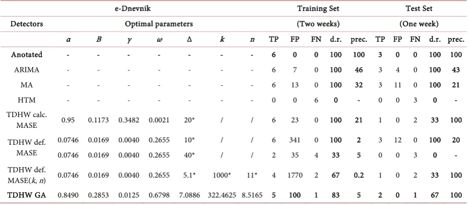
In Table 6 below are shown experiments for double seasonality for both

training sets and test sets for NEIS data.

The last rows indicated by gray color show the results of our HW GA. As can be seen in all the cases it outperforms or is equal to the results of the other algo-rithms. Direct comparison of the result achieved on the same benchmark data-sets can be done between proposed HW GA algorithm and HTM anomaly de-tection algorithm [5] (online implemented in [1]). HW GA and HTM have given equally good results on NUMENTA datasets, while HW GA (100% detection rate and 0% false positive) significantly outperform HTM on all the Yahoo benchmark datasets as also our e-dnevnik dataset. HW GA outperforms the best results (detection rate 84.67%, and false positive 10.12%) of HW forecasting al-gorithm with parameter maximum likelihood estimates optimization in [53], as also results of another type of algorithms (sliding windows) applied on the simi-lar type of data streams reported in [6].

The other important achievement of the HW GA [1] is that the algorithm is self-learning and can be implemented as a positive feedback optimization with a periodic adaptation of the parameters of the algorithm. In Table 2 the first data-set is used as a training data-set. Anomalies detected on the second datadata-set (test data-set) are verified/acknowledged by human and reused for new parameter optimiza-tion. With such newly optimized parameters detection is implemented on the third set and so on.

Correct results are achieved even in the case when there are no anomalies in the training set, while the test set has anomalies (example in Table 3).

In Tables 3-6 below, the parameters used by various algorithms are shown.

DOI: 10.4236/jcc.2019.78004 49 Journal of Computer and Communications

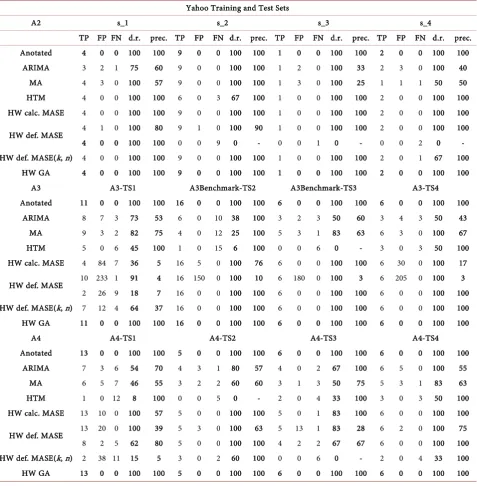
Table 2. The result from all tested algorithms for Yahoo benchmark (DR and precision). Yahoo Training and Test Sets

A2 s_1 s_2 s_3 s_4

TP FP FN d.r. prec. TP FP FN d.r. prec. TP FP FN d.r. prec. TP FP FN d.r. prec. Anotated 4 0 0 100 100 9 0 0 100 100 1 0 0 100 100 2 0 0 100 100

ARIMA 3 2 1 75 60 9 0 0 100 100 1 2 0 100 33 2 3 0 100 40 MA 4 3 0 100 57 9 0 0 100 100 1 3 0 100 25 1 1 1 50 50 HTM 4 0 0 100 100 6 0 3 67 100 1 0 0 100 100 2 0 0 100 100 HW calc. MASE 4 0 0 100 100 9 0 0 100 100 1 0 0 100 100 2 0 0 100 100

HW def. MASE 4 1 0 100 80 9 1 0 100 90 1 0 0 100 100 2 0 0 100 100 4 0 0 100 100 0 0 9 0 - 0 0 1 0 - 0 0 2 0 - HW def. MASE(k, n) 4 0 0 100 100 9 0 0 100 100 1 0 0 100 100 2 0 1 67 100

HW GA 4 0 0 100 100 9 0 0 100 100 1 0 0 100 100 2 0 0 100 100 A3 A3-TS1 A3Benchmark-TS2 A3Benchmark-TS3 A3-TS4 Anotated 11 0 0 100 100 16 0 0 100 100 6 0 0 100 100 6 0 0 100 100

ARIMA 8 7 3 73 53 6 0 10 38 100 3 2 3 50 60 3 4 3 50 43 MA 9 3 2 82 75 4 0 12 25 100 5 3 1 83 63 6 3 0 100 67 HTM 5 0 6 45 100 1 0 15 6 100 0 0 6 0 - 3 0 3 50 100 HW calc. MASE 4 84 7 36 5 16 5 0 100 76 6 0 0 100 100 6 30 0 100 17

HW def. MASE 10 233 1 91 4 16 150 0 100 10 6 180 0 100 3 6 205 0 100 3 2 26 9 18 7 16 0 0 100 100 6 0 0 100 100 6 0 0 100 100 HW def. MASE(k, n) 7 12 4 64 37 16 0 0 100 100 6 0 0 100 100 6 0 0 100 100 HW GA 11 0 0 100 100 16 0 0 100 100 6 0 0 100 100 6 0 0 100 100

A4 A4-TS1 A4-TS2 A4-TS3 A4-TS4

Anotated 13 0 0 100 100 5 0 0 100 100 6 0 0 100 100 6 0 0 100 100 ARIMA 7 3 6 54 70 4 3 1 80 57 4 0 2 67 100 6 5 0 100 55

MA 6 5 7 46 55 3 2 2 60 60 3 1 3 50 75 5 3 1 83 63 HTM 1 0 12 8 100 0 0 5 0 - 2 0 4 33 100 3 0 3 50 100 HW calc. MASE 13 10 0 100 57 5 0 0 100 100 5 0 1 83 100 6 0 0 100 100

HW def. MASE 13 20 0 100 39 5 3 0 100 63 5 13 1 83 28 6 2 0 100 75 8 2 5 62 80 5 0 0 100 100 4 2 2 67 67 6 0 0 100 100 HW def. MASE(k, n) 2 38 11 15 5 3 0 2 60 100 0 0 6 0 - 2 0 4 33 100 HW GA 13 0 0 100 100 5 0 0 100 100 6 0 0 100 100 6 0 0 100 100

Table 3. Part of Numenta training set and test set optimal parameters. NUMENTA Benchmark

art_daily_flatmiddle 1 - 7 Training set 8 - 14 Test set

Anotated 0 0 0 1 0 0

HTM 0 0 0 1 0 0

α Β γ δ k n TP FP FN TP FP FN

HW calc. MASE 0.2209222 0.01034794 0.3481637 22* / / 0 0 0 1 0 0

DOI: 10.4236/jcc.2019.78004 50 Journal of Computer and Communications Continued

0.730153 0 0.02568603 25* / / 0 0 0 1 0 0 HW def. MASE(k, n) 0.730153 0 0.02568603 4.5* 150* 4* 0 0 0 1 0 0 HW GA 0.1415149 0.2648334 0.2101766 3.143707 75.26209 6.844539 0 0 0 1 0 0

Table 4. Part of Yahoo training set and test set optimal parameters.

Yahoo Webscope_S5

A3Benchmark A3-TS1 A3-TS2 A3-TS3 A3-TS4

Anotated 11 0 0 16 0 0 6 0 0 6 0 0

HTM 5 0 6 1 0 15 0 0 6 3 0 3

HW calc.

MASE 0.95 0.1173 0.3481 1* / / 4 84 7 16 5 0 6 0 0 6 30 0

HW def. MASE

0.1548 0.1163 0.0433 0.1* / / 10 233 1 16 150 0 6 180 0 6 205 0 0.1548 0.1163 0.0433 0.5* / / 6 124 5 16 60 0 6 18 0 6 100 0 0.1548 0.1163 0.0433 1* / / 2 44 9 16 0 0 6 0 0 6 9 0 0.1548 0.1163 0.0433 1.2* / / 2 26 9 16 0 0 6 0 0 6 0 0 HW def.

MASE(k, n) 0.1548 0.1163 0.0433 0.9* 12* 8* 7 12 4 16 0 0 6 0 0 6 0 0 HW GA 0.7120 0.6217 0.1068 2.2235 15.6346 4.744 11 0 0 16 0 0 6 0 0 6 0 0

Table 5. e-Dnevnil training set and test set TDHW GA optimal parameters.

e-Dnevnik Training Set Test Set

Detectors Optimal parameters (Two weeks) (One week)

α Β γ ω Δ k n TP FP FN d.r. prec. TP FP FN d.r. prec. Anotated - - - 6 0 0 100 100 3 0 0 100 100

ARIMA - - - 6 7 0 100 46 3 4 0 100 43 MA - - - 6 13 0 100 32 3 11 0 100 21

HTM - - - 0 0 6 0 - 0 0 3 0 -

TDHW calc.

MASE 0.95 0.1173 0.3482 0.0021 20* / / 6 23 0 100 21 1 0 2 33 100 TDHW def.

MASE

0.0746 0.0169 0.0040 0.2655 10* / / 6 341 0 100 2 3 12 0 100 20 0.0746 0.0169 0.0040 0.2655 40* / / 2 35 4 33 5 0 0 3 0 - TDHW def.

MASE(k, n) 0.0746 0.0169 0.0040 0.2655 5.1* 1000* 11* 4 1770 2 67 0.2 1 0 2 33 100 TDHW GA 0.8490 0.2853 0.0125 0.6798 7.0886 322.4625 8.5165 5 100 1 83 5 2 0 1 67 100

Table 6. Percentage of TP anomalies found depending on and the GA iteration.

e-Dnevnik Training Set Test Set

Detectors Optimal parameters (Two weeks) (One week) α Β γ Δ k n TP FP FN d.r. prec. TP FP FN d.r. prec. Anotated - - - 6 0 0 100 100 3 0 0 100 100

DOI: 10.4236/jcc.2019.78004 51 Journal of Computer and Communications Continued

MA - - - 6 13 0 100 32 3 11 0 100 21

HTM - - - 0 0 6 0 - 0 0 3 0 -

HW calc.

MASE 0.95 0.0487 0.3482 10* / / 6 230 0 100 3 3 3 0 100 50

HW def. MASE

0.6579 0 0 10* / / 6 230 0 100 3 3 3 0 100 50 0.6579 0 0 20* / / 5 50 1 83 9 1 0 2 83 100 0.6579 0 0 30* / / 3 10 3 50 23 1 0 2 50 100 0.6579 0 0 40* / / 2 4 4 33 33 0 0 3 33 - HW def.

MASE(k, n) 0.6579 0 0 3* 115* 10* 3 13 3 50 18.8 3 30 0 50 9 HW GA 0.4075 0.5093 0.5325 7.2826 330.6001 11.0024 6 0 0 100 100 3 0 0 100 100

5. Conclusions

As a conclusion, we may say that anomaly detection in real-time massive data streams nowadays is very important in different domains. From the reviewed and classified literature, we came to the conclusion that there is a broad research area, covering mathematical, statistical, information theory methodologies for anomaly detection. A big number of methods (distance-based, clustering, classi-fication, machine learning, predictive based) coming from these areas are in re-lation with the various factors and problems of anomaly detection we have (the type of data, type of anomaly, availability of annotated anomalies in training set).

In this paper, we restricted ourselves to study algorithms for anomaly detec-tion in data streams (time series data) due to problem area we investigate ano-maly detection in log files streams.

In order to choose the appropriate algorithm, we have studied several algo-rithms suitable for anomaly detection in real-time massive data streams from where we chose to further test several of them (MA, ARIMA, HTM) and togeth-er with standard HW and TDHW to propose our algorithm as a future work.

DOI: 10.4236/jcc.2019.78004 52 Journal of Computer and Communications the national online educational system.

Availability of Data and Material

The dataset used in this paper is offered by FINKI data center for research pur-poses, they are data from e-dnevnik (national education system in Macedonia). Link: http://ednevnik.edu.mk/.

Authors’ Contributions

Jakup Fondaj has done the review of existing algorithms and also was part of ex-ecuting experiments. Zirije Hasani proposes the new adaptive algorithm.

Conflicts of Interest

The authors declare no conflicts of interest regarding the publication of this pa-per.

References

[1] Hasani, Z., Jakimovski, B., Velinov, G. and Kon-Popovska, M. (2018) An Adaptive Anomaly Detection Algorithm for Periodic Real Time Data Streams. In: Interna-tional Conference on Intelligent Data Engineering and Automated Learning, Sprin-ger, Berlin, 385-397.

[2] Hyndman, R.J. and Athanasopoulos, G. (2018) Forecasting: Principles and Practice. 2nd Edition, Texts Monash University, Lexington.

[3] Ekberg, J., Ylinen, J. and Loula, P. (2011) Network Behaviour Anomaly Detection Using Holt-Winters Algorithm. 6th International Conference on Internet Technol-ogy and Secured Transactions, IEEE, Piscataway, 627-631.

[4] Shahin, A.A. (2016) Using Multiple Seasonal Holt-Winters Exponential Smoothing to Predict Cloud Resource Provisioning. International Journal of Advanced Com-puter Science and Applications, 7, 91-96.

https://doi.org/10.14569/IJACSA.2016.071113

[5] Ahmad, S. and Purdy, S. (2016) Real-Time Anomaly Detection for Streaming Ana-lytics. 1-10.

[6] Li, G., Wang, J., Liang, J. and Yue, C.T. (2018) The Application of a Double CUSUM Algorithm in Industrial Data Stream Anomaly Detection. Symmetry, 10, 2-14.https://doi.org/10.3390/sym10070264

[7] Cortez, P., Rocha, M. and Neves, J. (2001) Genetic and Evolutionary Algorithms for Time Series Fore-Casting. In: Monostori, L., Váncza, J. and Ali, M., Eds., Engineer-ing of Intelligent Systems, Lecture Notes in Computer Science, Vol. 2070, SprEngineer-inger, Berlin, Heidelberg, 393-402.https://doi.org/10.1007/3-540-45517-5_44

[8] Agapie, A. and Agapie, A. (1997) Forecasting the Economic Cycles Based on an Ex-tension of the Holt-Winters Model. A Genetic Algorithms Approach. Computa-tional Intelligence for Financial Engineering, Proceedings of the IEEE/IAFE, New York, 24-25 March 1997, 96-99.

[9] Eusébio, E., Camus, C. and Curvelo, C. (2015) Metaheuristic Approach to the Holt-Winters Optimal Short Term Load Forecast. Renewable Energy and Power Quality Journal, 10, 708-713.https://doi.org/10.24084/repqj13.460

DOI: 10.4236/jcc.2019.78004 53 Journal of Computer and Communications Swarm Optimization in Forecasting Exchange Rates. Journal of Computers, 11, 216-224.https://doi.org/10.17706/jcp.11.3.216-224

[11] de Assis, M.V.O., Carvalho, L.F., Rodrigues, J.J.P.C. and Proença, M.L. (2013) Holt-Winters Statistical Forecasting and ACO Metaheuristic for Traffic Characteri-zation. IEEE International Conference on Communications, Budapest, 2524-2528. https://doi.org/10.1109/ICC.2013.6654913

[12] NUMENTA Anomaly Benchmark with Labeled Anomalies.

https://github.com/numenta/NAB/tree/master/data/artificialWithAnomaly

[13] Hamamoto, A.H., Carvalho, L.F., Sampaio, L.D.H., Abrao, T. and Proencüa Jr., M.L. (2017) Network Anomaly Detection System Using Genetic Algorithm and Fuzzy Logic. Expert Systems with Applications: An International Journal, 99, 390-402. https://doi.org/10.1016/j.eswa.2017.09.013

[14] Scrucca, L. (2013) GA: A Package for Genetic Algorithms in R. Journal of Statistical Software, 53, 1-37. https://doi.org/10.18637/jss.v053.i04

[15] Yahoo: S5—dA Labeled Anomaly Detection Dataset, Version 1.0(16M).

https://webscope.sandbox.yahoo.com/catalog.php?datatype=s%5c&did=70

[16] Pokrajac, D., Lazarevic, A. and Latecki, L.J. (2007) Incremental Local Outlier Detec-tion for Data Streams. IEEE Symposium on ComputaDetec-tional Intelligence and Data Mining, Honolulu, 1 March-5 April 2007, 1-12.

https://doi.org/10.1109/CIDM.2007.368917

[17] Weigend, A.S., Mangeas, M. and Srivastava, A.N. (1995) Nonlinear Gated Experts for Time-Series—Discovering Regimes and Avoiding over Thing. International Journal of Neural Systems, 6, 373-399.https://doi.org/10.1142/S0129065795000251

[18] Salvador, S., Chan, P. and Brodie, J. (2004) Learning States and Rules for Time Se-ries Anomaly Detection. American Association for Artificial Intelligence, Mel-bourne.

[19] Shekhar, S., Lu, C.T. and Zhang, P. (2001) Detecting Graph-Based Spatial Outliers: Algorithms and Applications (A Summary of Results). In: Proceedings of the 7th ACM SIGKDD International Conference on Knowledge Discovery and Data Min-ing, ACM Press, New York, 371-376.https://doi.org/10.1145/502512.502567

[20] Song, X.Y., Wu, M.X., Jermaine, C. and Ranka, S. (2007) Conditional Anomaly De-tection. IEEE Transactions on Knowledge and Data Engineering, 19, 631-645. https://doi.org/10.1109/TKDE.2007.1009

[21] Warrender, C., Forrest, S. and Pearlmutter, B. (1999) Detecting Intrusions Using System Calls: Alternate Data Models. In: Proceedings of the 1999 IEEE ISRSP, IEEE Computer Society, Washington DC, 133-145.

[22] Sun, P., Chawla, S. and Arunasalam, B. (2006) Mining for Outliers in Sequential Databases. SIAM International Conference on Data Mining, Sydney, 21 January 2006, 94-105.

https://doi.org/10.1137/1.9781611972764.9

[23] Chan, P.K. and Mahoney, M.V. (2005) Modeling Multiple Time Series for Anomaly Detection. In: Proceedings of the 5th IEEE International Conference on Data Min-ing, IEEE Computer Society, Washington DC, 90-97.

[24] Noble, C.C. and Cook, D.J. (2003) Graph-Based Anomaly Detection. Data Mining and Knowledge Discovery, 29, 625-688.https://doi.org/10.1145/956750.956831

[25] Phua, C., Lee, V., Smith, K. and Gayler, R. (2004) A Comprehensive Survey of Data Mining-Based Fraud Detection Research. CoRR 1009(6119), 1-14.

DOI: 10.4236/jcc.2019.78004 54 Journal of Computer and Communications CRC Press, Taylor & Francis Group, Boca Raton, London, New York.

[27] Sreevidya, S.S., et al. (2014) A Survey on Outlier Detection Methods. International Journal of Computer Science and Information Technologies, 5, 8153-8156.

[28] Gogoi, P., Bhattacharyya, D.K., Borah, B. and Kalita, J.K. (2011) A Survey of Outlier Detection Methods in Network Anomaly Identification. The Computer Journal, 54, 570-588.https://doi.org/10.1093/comjnl/bxr026

[29] Ranshous, S., Shen, S., Koutra, D., Faloutsos, C. and Samatova, N.F. (2013) Anoma-ly Detection in Dynamic Networks: Survey. WIREs Computational Statistics, 7, 223-247.https://doi.org/10.1002/wics.1347

[30] Zwietasch, T. (2014) Detecting Anomalies in System Log Files Using Machine Learning Techniques. Bachelor Thesis, University of Stuttgart, Stuttgart.

[31] Viaene, S. (2014) Analysis and Evaluation of Anomaly Detection Methods in Inte-grated Management. Master Thesis, EPFL, Lausanne.

[32] Goldstein, M. and Uchida, S. (2016) A Comparative Evaluation of Unsupervised Anomaly Detection Algorithms for Multivariate Data. PLoS ONE, 11, e0152173. https://doi.org/10.1371/journal.pone.0152173

[33] Simple Guide to Confusion Matrix Terminology.

https://www.dataschool.io/simple-guide-to-confusion-matrix-terminology

[34] Median Absolute Deviation of Moving Windows RunMAD.

http://veda.cs.uiuc.edu/TCGA_classify/RWR/DRaWR/library/caTools/html/runma d.html

[35] Boxplot. https://www.r-statistics.com/tag/boxplot-outlier [36] Twitter Advec. https://github.com/twitter/AnomalyDetection [37] MAD and DBSCAN Algorithms.

https://www.datadoghq.com/blog/outlier-detection-algorithms-at-datadog

[38] DBSCAN. https://cran.r-project.org/web/packages/dbscan/dbscan.pdf

[39] Kasunic, M., McCurley, J., Goldenson, D. and Zubrow, D. (2012) An Investigation of Techniques for Detecting Data Anomalies in Earned Value Management Data. Carnegie Mellon University, 3, 2-103.https://doi.org/10.21236/ADA591417

[40] Moving Range Technique. https://gist.github.com/tomhopper/9000495 [41] Moving Range Technique.

http://qualityamerica.com/LSS-Knowledge-Center/statisticalprocesscontrol/moving

_range_chart_calculations.php

[42] Moving Average.

https://cran.r-project.org/web/packages/smooth/vignettes/sma.html

[43] Gooijer, J.G. and Hyndman, R. (2006) 25 Years of Time Series Forecasting. Interna-tional Journal of Forecasting, 22, 443-473.

https://doi.org/10.1016/j.ijforecast.2006.01.001

[44] Brutlag, J.D. (2000) Aberrant Behavior Detection in Time Series for Network Mon-itoring. In: Proceedings of the 14th USENIX Conference on System Administration, ACM, Louisiana, 139-146.

[45] Galvas, G. (2016) Time Series Forecasting Used for Real-Time Anomaly Detection on Websites. Master Thesis, Vrije Universiteit, Amsterdam.

[46] Nur Intan Liyana Binti Mohd Azmi (2013) Parameters Estimation of Holt-Winter Smoothing Method Using a Genetic Algorithm. Master Thesis, Universiti Teknolo-gi, Malaysia.

DOI: 10.4236/jcc.2019.78004 55 Journal of Computer and Communications Constants-Does Solver Really Work? American Journal of Business Education, 6, 347-360.https://doi.org/10.19030/ajbe.v6i3.7815

[48] Yusuf Ziya Ünal at all (2015) Developing Spreadsheet Models of Holt-Winter Me-thods and Solving with Microsoft Excel Solver and Differential Evaluation Tech-nique: An Application to Tourism Sector. Proceedings of the 2015 International Conference on Industrial Engineering and Operations Management Dubai, United Arab Emirates (UAE), Dubai,3-5 March 2015.

[49] Md Maarof, M.Z., Ismail, Z. and Fadzli, M. (2014) Optimization of SARIMA Model Using Genetic Algorithm Method in Forecasting Singapore Tourist Arrivals to Ma-laysia. Applied Mathematical Sciences, 8, 8481-8491.

https://doi.org/10.12988/ams.2014.410847

[50] Hasani, Z. and Fondaj, J. (2018) Improvement of Implemented Infrastructure for Streaming Outlier Detection in Big Data with ELK Stack. In: Rocha, Á., Adeli, H., Reis, L.P. and Costanzo, S., Eds., 6th World Conference on Information Systems and Technologies, Vol. 2, Springer, Berlin, 869-877.

https://doi.org/10.1007/978-3-319-77712-2_82

[51] Leys, C., Ley, C., Klein, O., Bernard, P. and Licata, L. (2013) Detecting Outliers: Do Not Use Standard Deviation around the Mean, Use Absolute Deviation around the Median. Journal of Experimental Social Psychology, 49, 764-766.

https://doi.org/10.1016/j.jesp.2013.03.013

[52] Hyndman, R.J. and Koehler, A.B. (2006) Another Look at Forecast-Accuracy Me-trics for Inter-Mittent Demand. International Journal of Forecasting, 22, 679-688. https://doi.org/10.1016/j.ijforecast.2006.03.001

[53] Andrysiak, T., Saganowski, Ł. and Maszewski, M. (2017) Time Series Forecasting Using Holt-Winters Model Applied to Anomaly Detection in Network Traffic. In-ternational Joint Conference, 649, 567-576.

https://doi.org/10.1007/978-3-319-67180-2_55

[54] Hasani, Z. (2017) Robust Anomaly Detection Algorithms for Real-Time Big Data: Comparison of Algorithms. In: 6th Mediterranean Conference on Embedded Computing, IEEE, Montenegro, 1-6.https://doi.org/10.1109/MECO.2017.7977130

List of Abbreviations

• _{ARMA—Auto Regressive Moving Average}

• _{ARIMA—AutoRegressive Integrated Moving Average} • _{TDHW—Taylor’s Double Holt-Winters}

• _{HW—Holt-Winters}

• _{NEIS—National education information system} • _{GA—Genetic Algorithm}

• _{MASE—Mean Absolute Scaled Error} • _{TP—True positive}